

Francesco’s Substack
We deployed an AI autoresearch agent to tune GLM-5.2 serving on our NVIDIA B200 cluster. It doubled throughput in 26 runs. Real production-shape traffic replay broke it at 4-minute TTFTs. We fixed it through a series of manually tuned configuration setup and obtained 18x faster first tokens, 442 tok/s/GPU peak, and pushed the latency/throughput pareto optimal by more than 2.2x in latency and +35% in throughput. While the agent got us 80% there on a cold-start, engineering discipline and production traffic simulations closed the gap.
---
The journey to bring GLM5.2 to our customers within the AI Foundation Service of T-Systems began a few weeks ago when we started experimenting with GLM5 on our brand-new NVIDIA B200 cluster built out in Munich. The excitement of testing brand-new hardware with an open-weights LLM totalling 744B parameters, hosted and served entirely on our own infrastructure, was palpable and, after a few iterations patching missing components on Day-1 of the release, we finally got “something” working. It was prompting, responding, responses seemed reasonable, we could see GPU usage, power spikes and all. Pretty exciting start! After a couple of measurements on our performance, ouch! We realized we still had a long way to go (expected, of course, but it still bites every time). But where to start, exactly?
Thanks for reading Francesco’s Substack! Subscribe for free to receive new posts and support my work.
Subscribe
Take for example the topology, i.e. how you decide to parallelize your model over the GPUs in your cluster: a 744B parameters model in NVFP4 (4-bit precision, roughly half-byte per parameter), takes around 372GB of GPU VRAM for weights alone, around 420GB once you include quantization scale factors. Every single B200 has around 183GB of HBM3e VRAM: two GPUs would give you 366GB, which is not enough for the 420GB of weights plus scales, so you need to split the model weights across no less than 3 GPUs. Considering you then need to leave room for the KV-cache pool, CUDA graphs and a bunch of other things, and considering the node is 8 GPUs and you don’t want to break something across 2 nodes (and you want to keep the power of 2 architecture of GPU clusters), then you are left in this case with splitting the model across 4 GPUs at minimum.
Also, say you are lucky enough to have for example 32 GPUs: now, you could have 8 replicas of 4 GPUs each introducing tensor parallelism equal 4, or you could have tensor parallelism equal 8 and 4 replicas, or tensor parallelism equal 4, data parallelism equal 2 and still 4 replicas. Then to this, you add inference engine: vLLM, SGLang or TensorRT-LLM? Should we use NVIDIA Dynamo or not? Should we deploy aggregated or disaggregated? While you see we have already piled up quite a few independent variables (say 4 topologies x 3 engines x 2 Dynamo on/off x 2 Agg/Disagg = 48 configurations to explore already...), we are just at the beginning: every engine has several configuration flags, more than 20, of which 10 at least are usually very important. For example, which attention backend, which kernels, how are the kernels compiled, the input sequence length, the maximum number of concurrencies, the memory occupancy, the size of the CUDA graphs to capture etc. etc. You can see how the number of configurations could easily exceed 2^10=1024 (assuming binary values), per engine flags alone!
So, where to start? Of course, brute force would just pile up each one of these configurations, automate benchmarking of each one of those (we’ll talk about this more later), and select the best ones. Considering each benchmark takes several minutes, the brute force approach would have taken weeks of cluster time, making it a dead idea from the start. There are also several tools to run “estimations” from scratch (like aiconfigurator), but on Day-0, you usually don’t have a lot of reliable data, except your own priors in the space. You can also be smart about it and apply Design of Experiments approach, running full or fractional factorial design, or Hadamard design, but even these statistical methods rely on arbitrary models of interactions that you create a-priori. We decided to test a brand-new idea from the community: an autoresearch agent inspired by the work of Andrej Karpathy.
The main idea about autoresearch is quite simple: you create a robust harness with verifiable outcome, and an automated procedure to iterate, and with a series of prompts, skills and agents defined (and in this case, a proper security context!), you solve the problem with agentic coding with e.g. Claude Code/Codex/OpenCode and your favorite LLM backend. You throw compute at the problem! Which is what we decided to do: we created a new autoresearch framework to launch from an autonomous pod on our Kubernetes cluster. The agent runs in a 4 stages-loop within the sandbox, fully separate from production and from any customer data. It operates in a dedicated namespace with non-privileged pods, resource quotas, and permissions scoped to deploying and benchmarking its own candidate configurations: the blast radius is its own sandbox, nothing else. First, the agent plans the next candidate configuration from the current best, by swapping one variable at a time, for example by changing precision, tensor parallelism, number of replicas, KV-cache data type, routing policy, disaggregated prefill/decode layout etc. Second, it deploys the selected configuration by auto creating the manifest with per-replica deployment, DRA resource claim (aligning GPUs with NIC cards), cache-aware routing and server arguments. The third step is evaluation of the rolled-out configuration with a synthetic performance benchmark at fixed-length of input and output generation and a fixed request rate. The final and fourth step is to report the results and updating the best configuration if it outperforms the current iteration’s top candidate. A crucial decision was to enable the agent to add a learning skill that auto updates at every cycle, documenting failure modes, root-cause analyses and proposing fixes to the found blocker.

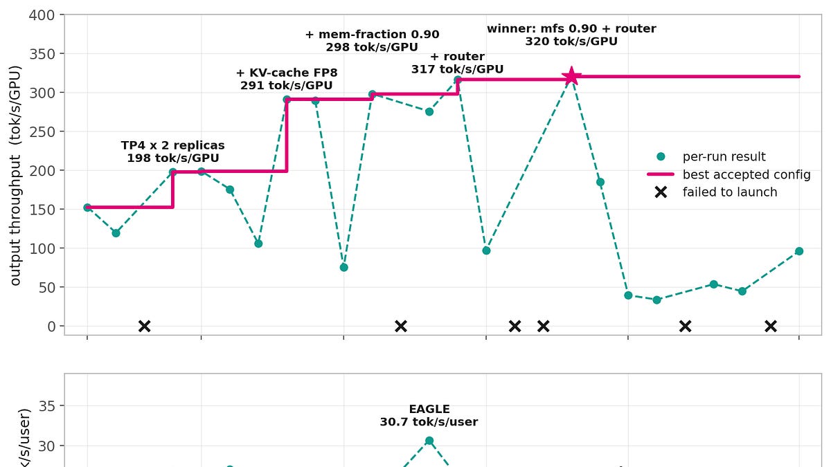
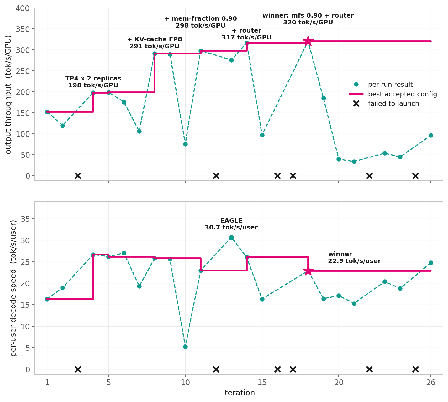
Figure 1. The autoresearch agent’s 26 iterations search on GLM5 shows each attempted configuration, the best configuration accepted at any given iteration, and configurations that failed to launch. We plot throughput per GPU, which is the metric the agent optimized, as well as per-user decode speed of the accepted config.
The autoresearch agent explored over 26 different configurations (Figure 1), and very importantly, we noticed the self-learning pattern was excluding entire families of configurations based on early failures. For example: run 3 tried FP8 at TP=4 and ran out of memory during weight re-quantization, therefore the agent wrote the lesson down as “FP8 requires TP=8 minimum on B200”, and in the 20+ runs that followed it never launched FP8 below TP=8 again. Same for NVFP4 quantization, which wouldn’t fit at TP=2, so “both quantization needs TP≥4” went into the knowledge base too, and no later run violated it. The failure notes restricted search by excluding forbidden configuration, ended early FP8 at TP=4 once it realized the smaller footprint of NVFP4 would make the model fit in 4 GPUs, tested the run which then became baseline to build the best configuration on top of. While these are obvious lessons to human engineers with sufficient experience in model inferencing, we found real value in the agentic capabilities to self-correct quickly and exclude entire families of configurations. While we haven’t tested previous generations of agentic models on the same task, we share the belief that this would have been hard to achieve e.g. 6 months ago.
Figure 1 reports the full sequence of experimental iterations. We see large gains early in the iterations, while the recipes stabilize after roughly 15 of the 26 runs. The two single major gains are given by switching to TP=4 (NVFP4 weights) and KV-Cache dtype in FP8: both optimizations reduce the model memory footprint and require less memory bandwidth. LLM decoding is dominated by memory traffic, since every generated token has to stream the weights and the KV-cache through the GPU. NVFP4 makes the model small enough to fit in 4 GPUs instead of 8, so the same hardware serves twice the replicas and each token pays the tensor-parallel all-reduce overhead across 4 GPUs instead of 8; the FP8 KV-Cache halves the bytes per cached token, which roughly doubles how many requests fit in a decode batch, and at saturation batch, size means throughput. The two further optimizations are relative to the memory fraction and a cache-aware router for better multi-pod routing within the cluster. The memory fraction is the share of GPU memory pre-reserved for weights plus the KV-Cache pool: raising it from 0.85 to 0.90 simply buys a larger KV pool, hence bigger decode batches, at the cost of headroom for everything else. The cache-aware router replaces the Kubernetes round-robin load balancer with SGLang’s own router, which tracks each replica’s queue depth and cached prefixes and sends every request where it will queue least and reuse the most KV; even on our synthetic prompts, which share no prefixes at all, the better load distribution alone increased throughput by roughly 8.8%. The interactivity plot shows a major gain in TP=4 and EAGLE speculative decoding, though this configuration was discarded because the agent was designed to optimize for throughput alone. Overall, the autoresearch agent increased the total throughput by 110% from 153 tok/s/GPU to 320 tok/s/GPU, and improved the interactivity by 40% from 16.3 tok/s/usr to 22.9 tok/s/usr.
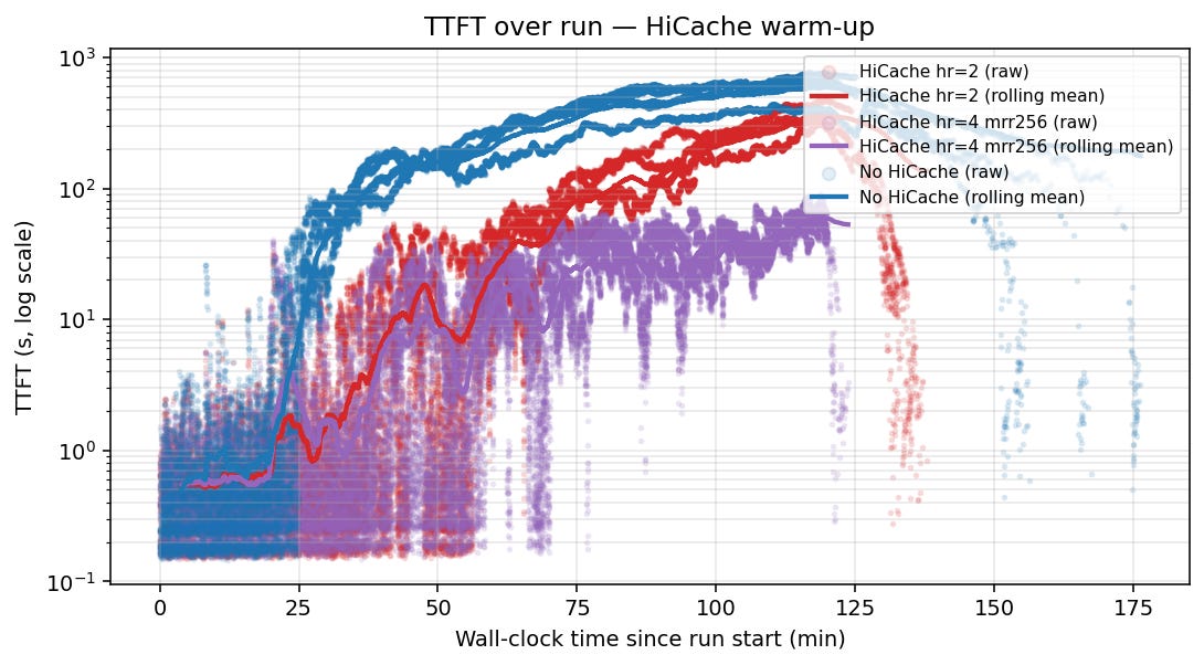
After the autoresearch agent completed its cycles (a few million tokens), we were excited of the improvement from the baseline configuration, especially regarding the throughput. However, an agent is as good as the harness one creates, and in this case, it had optimized for throughput under a simplified load-shape dictated by the benchmark we had created. It was time to put the configuration through a real test. We created our own mix of anonymized, production-derived LLM usage traces from the Qwen-Bailian Anonymous Dataset1: the dataset is released under Apache-2.0 license and contains production traces that are fully-anonymized via token-block hashing, domain remapping, ID randomization and time-based anonymization to ensure no PII, unlinkable by design and GDPR/CCPA compliant. Each trace is replayed with its own arrival time on a fixed schedule, which preserves the arrival shape into a production-like traffic load instead of smoothing it over in a Poisson process, as it normally is the case for synthetic benchmarks. We ran it through the best configuration, and, once again, ouch! We saw TTFT blow up to several minutes under realistic traffic bursts with variable prompt and generation lengths (blue line in Figure 2). A close inspection of the data and the log metrics we collected during the run, we observed the problem was an unbounded admission queue in the engine that blows up TTFT during bursty traffic replays.

Figure 2. Trace replay results in terms of wall-clock time vs TTFT of autoresearch configuration (baseline), HiCache, and combining HiCache and fixed maximum running requests.
Based on the observed behavior of uncapped concurrency, which was saturating the engine with bursty arrivals, we introduced two main axes of optimization: HiCache and maximum running requests.
The first dimension regards HiCache, which is a hierarchical KV-caching system from SGLang. HiCache allows you to avoid redundant computations by storing shared KV-caches (mostly prefixes and recurring prompts like system prompts or identical codebases for coding agents) by storing the RadixCache from the inference engine into multiple tiers of storage, such as local NVMe and parallel file systems or any other storage device or class available. The main parameter controlling its behavior is the HiCache ratio, which represents the ratio of the size of the KV-Cache memory pool to the size of the device pool. For example, a ratio of 4 implies that the caching pool on the host is 4 times larger than the one in the device. We were able to reduce the wall-clock of the trace replay by 22% (measured on the coder-only trace) while keeping the overall throughput unchanged by simply introducing a HiCache with a ratio of 2 (Figure 2).
The second dimension controls the request admission limit and is given by the maximum number of running requests allowed in the engine. SGLang for example calculates this parameter dynamically when it is not explicitly set it profiles the available GPU memory to determine the number of KV-Cache token slots, estimates the maximum number of running requests as (token slots / context length) × 512, and clamps the result into the 2048–4096 interval. The default tends to overestimate the concurrency an engine can realistically sustain. Observing the logged metrics, we found it caused over-admission: throughput had long plateaued while latency kept growing with every extra admitted request. After a few iterations we found a cap of 256 to hit the sweet spot, keeping admission close to the engine’s real capacity. We combined the capped request with a HiCache ratio of 4, since we noticed that roughly a third of the evicted tokens were being reused at a HiCache ratio of 2.
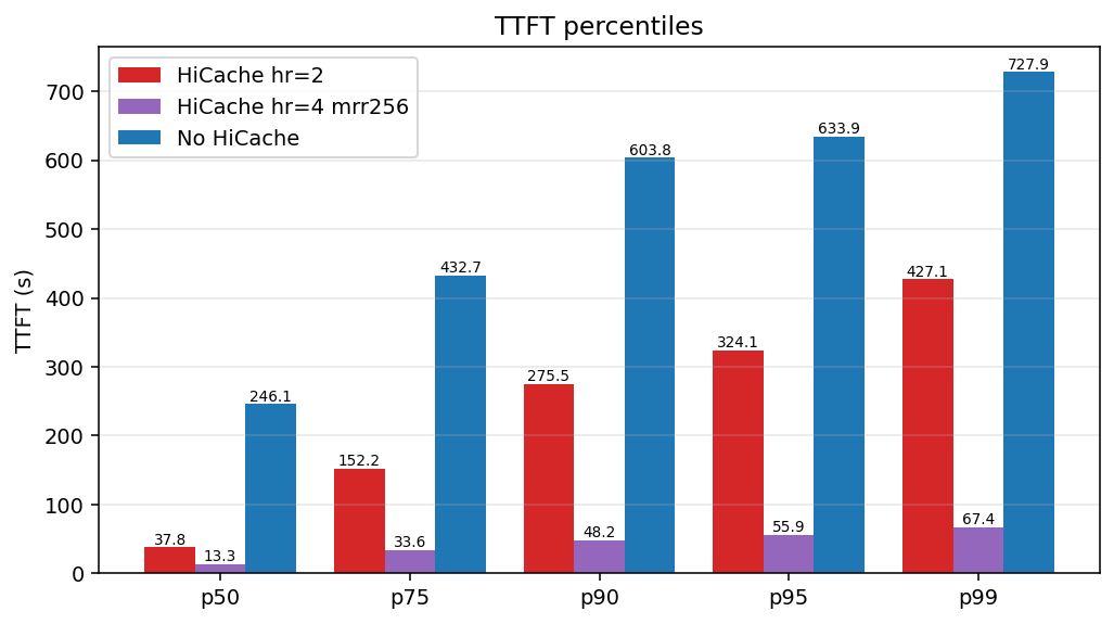
The combined measures allowed us to drastically reduce the wall-clock time of the trace replay, and, most importantly, keep a relatively flat TTFT tail distribution, by reducing the p50 TTFT from 246.1 s to 13.3 s (18x improvement) and p99 TTFT from 727.9s to 67.4s (11x improvement). We further ran ablation studies on the capped request alone, and we found it to be the dominant variable in controlling the mean and variance of TTFT, reducing both averages and tail behavior.

Figure 3.TTFT percentiles of trace replay result of autoresearch configuration (baseline), HiCache alone, and combining HiCache and fixed maximum running requests.
---
As GLM5.2 became available for the community, we had all the recipes to deploy it efficiently on our infrastructure: the baseline recipe from autoresearch agent, and the manually tuned additions to sustain production-shaped traffic. We started by running a concurrency sweep from the optimal GLM5 configuration (by this time, we had it ported to GLM5.1) and settled the baseline pareto frontier from 4 to 256 concurrent requests in the interactivity vs throughput plot (Figure 4, magenta line). We found our configuration to massively outperform the autoresearch cold-start in both latency and throughput, covering a wide range of conditions based on the number of concurrent users on the cluster. We then noticed how the autoresearch agent had discarded the speculative decoding configurations (EAGLE) as it was maximizing purely on throughput. We decided to further explore and, after a few manual tuning of the parameters (including graph capture size, memory and a further adjustment of maximum running requests), we found that speculative decoding was extending the interactivity frontier from 92 to 202 tok/s/usr at low concurrency (Figure 4), a 2.2x increase, albeit reducing the peak throughput by 25%, from 436 down to 327 tok/s/GPU at high concurrency. As expected, speculative decoding trades lower latency for a lower throughput. However, we decided to further test adaptive speculative decoding, which adapts the ratio between how many draft-model autoregressive steps run in each speculative round and the number of draft tokens verified per step. After another set of tuning iterations, we found that adaptive speculative decoding was keeping intact the high-interactivity at low concurrency (198 vs 202 tok/s/usr at concurrency 4, within 2.5% of fixed speculative decoding), while further recovering the full throughput of the best configuration without speculative decoding: at concurrency 128 it reaches 442 tok/s/GPU, a 35% peak-throughput lift over fixed speculative decoding (327 tok/s/GPU) and even slightly above the non-speculative baseline (436 tok/s/GPU). The pareto frontier is extended at both ends, and the trade-off effectively disappears.

Figure 4. Pareto frontier of throughput vs interactivity across the optimization journey. GLM5 autoresearch points were measured under the agent’s saturated synthetic benchmark; GLM5.2 curves come from production concurrency sweeps.
From the first working configuration to what serves customers today, the throughput per GPU almost tripled from 153 tok/s/GPU on day 0, to 442 tok/s/GPU at peak now. The median TTFT under production-shaped traffic fell from 246 s to 13.3 s, an 18× drop, and the p99 tail from 728 s to 67 s. Finally, interactivity at low concurrency went from 16 tok/s/usr on day 0, to 198 tok/s/usr without sacrificing any peak throughput thanks to adaptive speculative decoding.
---
The first thing that came to mind, is Richard Sutton’s bitter lesson: learning and search via raw compute are often outperforming human-based heuristics. In this case, the agentic AI approach with a properly human-designed harness allowed us to quickly and efficiently scan a very large space of configurations to get a model performing well-enough for day-0 scenario. Leveraging compute in the form of tokens, the agent was able to weed out all the ill-conceived configuration and discard entire families of optimization based on the learning.
We also quickly realized how any agent is as good as the harness and targets you set for it, and something that was optimized for a synthetic benchmark, was of course not delivering an engine tuned for a production-shaped traffic. The anonymized trace replays played a fundamental role in understand what was needed from the configuration to be able to sustain a real use case.
Our study is a good example of how engineering judgement acts as complementary support to AI-driven development; the two modes are not in antithesis, but one constitutes the synthesis of the other. The engineering context, i.e., most of the technical conversations we had as a team, the experience we built and the result of our outgoing activities of reading blogs, papers, posts and other material, was something that a boxed AI agent won’t be able to incorporate. We believe agentic AI is a boost to the engineering work, not a replacement.
Through this work, we also observed how many big and early achievements in performance optimization are mostly on a configuration level. As we are approaching the physical limits of what pure configuration tuning can do, we will now start to investigate kernels and optimized strategies for data movement (it usually boils down to that).
GLM5.2 is now live with our customer base, and we are closely monitoring the performance in real time. Real traffic is the ultimate benchmark, and as adoption ramps up we are already investing in the next round of improvement (hint: yes, it will be disaggregated serving!) so that our service levels keep holding as more users join. Going live early is proving to be the right decision: our assumptions are turning from educated guesses into direct observation.
Every step has taught us important lessons on search, tuning, battle-testing and how assumptions, the foundation of any engineering design, need realignment once real data is presented. Throughout every step, we exercised engineering discipline by measuring but left room for creativity in exploring new ideas such as agentic-driven optimization. The recipe that emerged highlights the complementarity between human engineering and AI, and not the often-claim juxtaposition of one against the other. As we tackle the next round of more specialized optimization, we carry these lessons forward to further accelerate frontier model inference on our stack.
---
If this made you curious, most of what we used is public and you can get surprisingly far in one (or a few…) afternoon. The anonymized Qwen-Bailian traces we replayed are open, SGLang and its HiCache documentation are open. If there is enough interest, we’ll consider open-sourcing the autoresearch harness too, just tell us! If you are serving large MoE models, we’d genuinely like to hear about it: LinkedIn.
Wang, J., Han, J., Wei, X., Shen, S., Zhang, D., Fang, C., Chen, R., Yu, W. and Chen, H., 2025. KVCache Cache in the Wild: Characterizing and Optimizing KVCache Cache at a Large Cloud Provider. In 2025 USENIX Annual Technical Conference (USENIX ATC 25) (pp. 465-482).