Fourier pixels for bidirectional light control

Abstract

Digital cameras1.") and displays2.") use picture elements (pixels3.")) that perform a single function: detecting or emitting light intensity. To exploit the full information content of electromagnetic waves, more advanced elements are required. This has driven the development of multifunctional components that, for example, simultaneously detect and emit intensity4."),5.") or extract intensity and spectral information6."),7."),8."). However, no pixel exists that both senses and generates optical wavefronts with full control over amplitude, phase and polarization, limiting bidirectional control and feedback of sophisticated light fields. Here we present a route to such pixels by demonstrating a versatile platform of miniaturized diffractive elements based on Fourier optics9."). We use plasmonic surface waves10."), which propagate coherently11.") and efficiently12."),13."),14."),15.") across metallic surfaces. When these plasmons are launched towards wavy microstructures16.") designed with simple Fourier analysis, arbitrary and background-free optical wavefronts are generated. Conversely, incoming light can be sensed, and its amplitude, phase and polarization can be fully characterized. By combining or superposing several such components, we create multifunctional ‘Fourier pixels’ that provide compact and accurate control over the optical field. Our approach, which we extend to photonic waveguide modes, establishes a scalable, universal architecture for vectorially programmable pixels with applications in adaptive optics17."),18."), holographic displays19."),20."),21."), optical communication22."),23.") and quantum information processing24.").

Integrated metasurfaces for re-envisioning a near-future disruptive optical platform

Article Open access 20 June 2023

Optical meta-waveguides for integrated photonics and beyond

Article Open access 22 November 2021

Double-phase metasurface operators for all-optical image processing

Article Open access 23 February 2026

Main

Cameras1.") and displays2.") rely on picture elements (pixels3.")) that locally measure or emit light intensity. Similarly, spatial light modulators25.") (SLMs) contain pixels that alter the optical phase. Yet these elements modify only one property of light. Information is carried in its amplitude, phase and polarization. Thus, pixels that can generate and sense light with full control of these parameters would enable powerful multifunctional and bidirectional elements.

One possible route to such devices is to shrink Fourier optics9."), which is conventionally performed with bulky components. Metasurfaces26.")—arrays of nanoscale resonators that collectively control optical wavefronts—offer the ability to incorporate functionality in thin structures. Polarization cameras27."), phase detectors28."), phase modulators29."),30.") and various optical sources21."),31."),32."),33.") have been demonstrated. In addition, by intentionally coupling the nanoscale resonators, ‘non-local’ metasurfaces can emulate Fourier optics34."),35."). This has led to sources36.") and lasers37.") with full control over amplitude, phase and polarization.

However, no metasurface (local or non-local; large array or ‘pixel-sized’) has provided full bidirectional control. This is attributable in part to the limitations of metasurfaces. In general, light interacts with waves (sinusoids) in the interfacial profile. As metasurfaces approximate these sinusoids with discrete subwavelength resonators, higher functionality becomes increasingly difficult because many overlapping sinusoids must be represented simultaneously. Moreover, the design process is non-intuitive and computationally intensive38."). Numerical simulations must iteratively determine both local and non-local responses of the resonators to select their shapes and placements within the array. The design landscape is often rugged, prohibiting reliable convergence on an optimal solution.

The above limitations are rooted in a fundamental assumption of the metasurface approach: the surface must consist of ‘blocky’ discrete resonators because better-suited ‘wavy’ interfaces cannot be fabricated. In fact, diffractive interfaces that contain precise sums of sinusoids (known as Fourier surfaces) are possible16."). Because of their arbitrarily wavy profiles, they are ideally suited to control electromagnetic waves. Further, their design involves Fourier analysis, which is not only straightforward but also allows surface profiles for different tasks to be superposed. Thus, Fourier surfaces provide a direct route to Fourier optics in a small footprint. Here we exploit this direct Fourier approach to create a broad class of multifunctional ‘Fourier pixels’ that can generate and detect optical fields with arbitrary amplitude, phase and polarization.

Working principle of Fourier pixels

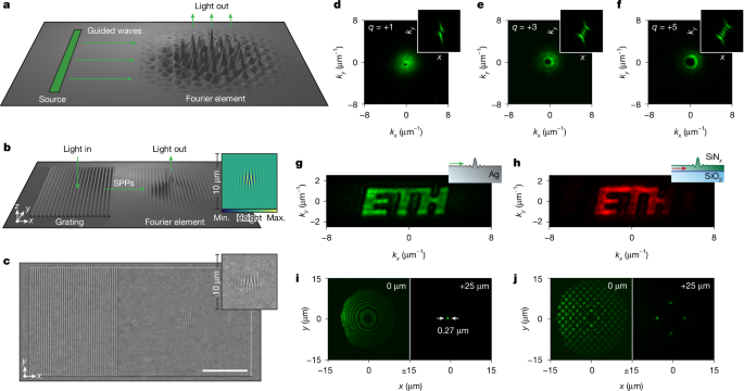
We define a Fourier pixel as a collection of precisely constructed interfacial components that perform a desired task with guided waves (Fig. 1a). We primarily use surface plasmon polariton (SPP) waves10."), which propagate coherently11.") and efficiently13.") across a metallic interface, but we also exploit photonic waveguide modes below. When these waves are launched from a source towards the primary design element (which we name the Fourier element), a precise, background-free optical field is outcoupled. For light shaping, this output is the desired optical wavefront emitted by the Fourier element. Alternatively, if the guided waves are generated at the source by an incoming optical wave, the output from the Fourier element can fully characterize this incoming light with the surface waves as intermediaries. Moreover, several surface profiles can be superposed within the same Fourier element to obtain multifunctionality. Thus, this simple architecture provides a thin, modular, scalable and universal platform for vectorially programmable bidirectional devices that both shape and sense light fields within footprints comparable to conventional pixels. Such sophisticated designs are only possible because wavy interfaces with accuracies of a few nanometres can be created16.").

Fig. 1: Fourier pixels for generating light with arbitrary amplitude and phase.

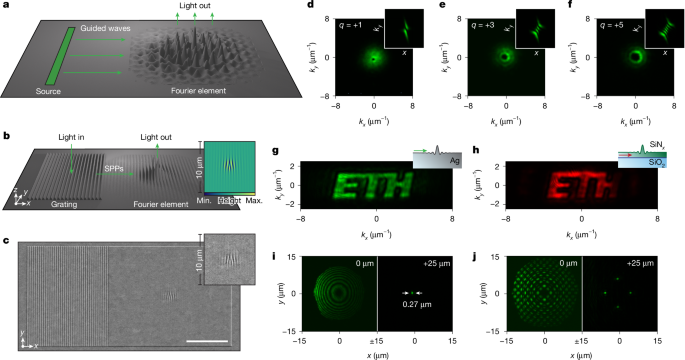
Fig. 1: Fourier pixels for generating light with arbitrary amplitude and phase.

Full size image

a, Concept of a Fourier pixel, including a source of surface guided waves, a propagation path and a diffractive Fourier element that generates an optical output. b, Plasmonic Fourier pixel that generates a Gaussian vortex beam with a topological charge of \$q=+1\$. The dimensions of the structures in a and b are exaggerated for clarity. The inset shows the surface profile (top view of the central region) required for the desired output. c, SEM of the structure depicted in b and its inset (35° tilt). Scale bar, 10 µm. d, Gaussian vortex beam with \$q=+1\$ from the Fourier pixel in c imaged at the back focal plane (Fourier plane) of an optical microscope. The dark centre of the beam profile indicates a phase singularity, confirmed by measured on-axis intensity less than 1% of the peak intensity. The value of \$q\$ is verified by inserting a cylindrical lens in the beam path (inset). e,f, Gaussian vortex beams imaged as in d with \$q=+3\$ (e) and \$+5\$ (f). Diagonal crosscuts of the cylindrical lens measurements exhibit intensity minima of 1–8% of the maximum intensity, indicating high twist-order purity with negligible contributions from unwanted orders. g,h, Experimental flat-phase images projected in Fourier space from a Ag (g) and SiN_x_ (h) Fourier pixel. i,j, Fourier pixels that generate a single diffraction-limited focal spot (i; s.d. = 0.27 µm) or a grid of foci (j) 25 μm above the Fourier pixel. For each case, the microscope is focused at the pixel plane (left; \$z=0\$ µm) and 25 µm above the pixel (right; \$z=25\$ µm). The wavelength was 555 nm for all devices except in h, which used 591 nm. Designs and SEM images for devices in e–j are shown in Extended Data Fig. 2. Max., maximum; min., minimum. Logo in g and h reproduced with permission from ETH Zurich (© 2026 ETH Zurich).

Fourier pixels for light generation

We first demonstrate plasmonic Fourier pixels that generate light with arbitrary amplitude and phase. We use silver (Ag) surfaces to maximize SPP propagation13."),39.") and pattern the entire device together to maintain phase relationships (Methods). The pixel in Fig. 1b creates a Gaussian beam with a twisted phase front that varies clockwise from \$0\$ to \$2{\\rm{\\pi }}\$ around the beam axis in the direction of propagation (known as a vortex beam with a topological charge, \$q\$, of \$+1\$). For simplicity, a sinusoidal grating (left) is used as the SPP source. Light incident with a specific energy and angle launches SPPs efficiently (approximately 70–80%; Methods). These SPPs then propagate in \$x\$ towards a diffractive Fourier element (right), which modifies them in three ways. It imprints the desired amplitude and phase profile on the outcoupled light and corrects the momentum mismatch between the SPPs and the emitted photons. Despite this complexity, the required design (Fig. 1b, inset) is easily determined by taking the inverse Fourier transform of the targeted complex-valued optical wavefront (amplitude and phase) while anticipating the required SPP-to-photon momentum change (Methods and Extended Data Fig. 1). Figure 1c shows a scanning electron micrograph (SEM) of the fabricated Fourier pixel. (Devices not shown in the main figures are presented in Extended Data Fig. 2, with design parameters given in Methods).

The pixel output is imaged with an optical microscope (Methods and Extended Data Fig. 3). A laser-cut mask is placed in the excitation path to selectively illuminate the grating. For convenience, all measurements below exploit coherent illumination, although incoherent excitation is also possible (Extended Data Fig. 4g). For the pixel in Fig. 1c, a characteristic ‘doughnut’ profile appears in the back focal plane (Fourier plane) of the microscope owing to the phase singularity at the centre of the vortex beam40.") (Fig. 1d). Using a cylindrical lens, which yields an interference pattern (Fig. 1d, inset) with \${|q|}\$ nodes and a tilt (right or left) that reveals the vortex handedness41."), we verify the topological charge (\$q=+1\$) of the beam. Figure 1e,f shows similar results for Fourier pixels that generate vortex beams with higher twist (\$q=+3\$ and \$+5\$). To further quantify the quality of the output, Fig. 1g presents a Fourier pixel (hologram) that projects a flat-phase image in Fourier space. The image exhibits uniform intensity with low speckle contrast (ratio of s.d. to mean intensity) of 17%, confirming the high fidelity of the imprinted phase, and an average signal-to-background ratio (ratio of mean intensity within the image to mean background averaged over the accessible numerical aperture) of 68, providing a conservative estimate of background suppression. Further examples of Fourier pixels that generate Hermite–Gaussian beams and project three-colour images are shown in Extended Data Fig. 4.

The Fourier pixels can also easily incorporate lensing functionality to place the desired output at arbitrary planes (not only in the Fourier plane). For example, by directly encoding a wavy Fresnel-type phase profile on a Fourier element, we create a single focal spot 25 μm above the pixel (Fig. 1i). The measured intensity distribution reveals a diffraction-limited focus (0.27 µm), indicating minimal aberration. Such pixels also confirm high throughput efficiency, with greater than 40% power-in to power-out for wavelengths from 500 nm to 700 nm (Methods). Extending this concept, Fig. 1j shows a grid of foci. Further results for outputs at arbitrary planes, including lenses with numerical apertures up to 0.8 and holograms projecting three-dimensional shapes, are presented in Extended Data Fig. 5.

However, full control of the emitted optical field requires manipulation of the polarization. Figure 2a shows a ‘vectorial’ Fourier pixel that uses two orthogonal gratings to launch SPPs with distinct wavevectors and in-plane polarizations. By coherently superposing the contributions from these two gratings, the Fourier element generates optical wavefronts with arbitrary amplitude, phase and polarization, enabling deterministic construction of emitted light fields. As an example, we launch SPPs with incident light polarized 45° with respect to each of the two orthogonal gratings (for equal amplitude in the two SPP paths) and create vector beams with polarization singularities. At the output Fourier plane, the field is constructed from the SPPs that originate from the \$x\$ and \$y\$ polarization projections of the two gratings (Fig. 2b). Figure 2c,d shows the output from Fourier pixels that generate first-order and second-order vector beams with the polarization rotating \$2{\\rm{\\pi }}\$ (Fig. 2b) and \$4{\\rm{\\pi }}\$ clockwise around the beam axis in the direction of propagation, respectively. The beam profile, with its dark centre and its evolution when a linear polarizer (analyser) is rotated in the detection path, confirms that the generated fields possess the targeted spatially varying polarization.

Fig. 2: Vectorial Fourier pixels for full light control and multiplexing.

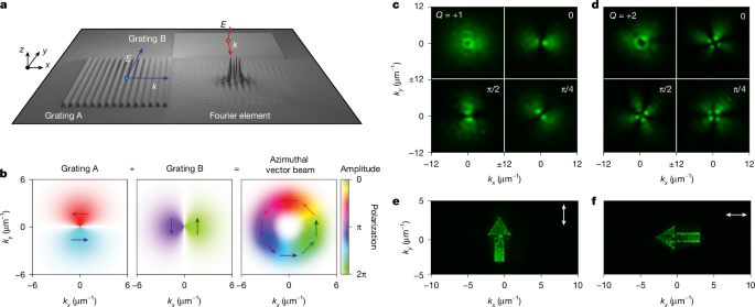
Fig. 2: Vectorial Fourier pixels for full light control and multiplexing.

Full size image

a, Vectorial Fourier pixel consisting of two orthogonal gratings and a Fourier element. Gratings A and B launch SPPs with orthogonal wavevectors and in-plane polarizations. The input waves from gratings A and B can be coherently superposed to generate light fields with arbitrary amplitude, phase and polarization. The dimensions of the structure are exaggerated for clarity. b, Construction of an azimuthally polarized vector beam is depicted. c,d, Experimental images of first-order (\$Q=+1\$) (c) and second-order (\$Q=+2\$) (d) vector beams in Fourier space without a linear polarizer in the detection path (top left) and with varying polarizer angles between \$0\$ and \${\\rm{\\pi }}/2\$. The polarization singularity introduces a dark hole in the vector beam. e,f, Polarization-multiplexed images of upward (e) and sideward (f) arrows. The separate images are selected by a linear polarizer (white arrow orientation) in the detection path. The wavelengths were 560 nm for c and d and 555 nm for e and f. Designs and SEM images for all devices are shown in Extended Data Fig. 2.

The ability to control polarization in the output enables multiplexing (Fig. 2e,f). By encoding two distinct images into orthogonal polarization states, a Fourier pixel can generate fields with different polarization using the same diffractive Fourier element. Rotation of an analyser in the detection path selectively reveals one image while suppressing the other, thereby establishing polarization-multiplexed image construction with negligible crosstalk.

Fourier pixels for light sensing

In addition to light generation, the same concepts can be exploited for sensing. Figure 3a illustrates a Fourier pixel that measures the phase difference \${\\varphi }\{{\\rm{in}}}\$ between light incident on two opposing sinusoidal gratings. These gratings launch counter-propagating SPPs towards a central Fourier element, designed to diffract the two outcoupled light fields together (Extended Data Fig. 6a). To determine \${\\varphi }\{{\\rm{in}}}\$ without a reference wave, the Fourier element also adds a phase difference \${\\varphi }\{{\\rm{out}}}\$ between the two light fields that depends on the outcoupled angle \$\\theta \$. The phase difference \${\\varphi }\{{\\rm{out}}}\$ varies from \$0\$ to \$2{\\rm{\\pi }}\$ and back to \$0\$ over a range of \$\\theta \$ (along \$x\$). This extra phase \${\\varphi }\{{\\rm{out}}}(\\theta )\$ (Fig. 3a, inset) results in constructive and destructive interference between the output waves as a function of \$\\theta \$. Consequently, at the output Fourier plane (Fig. 3b), two nodes arise from destructive interference at a specific angle \$\\theta \$. The Fourier element is also designed to outcouple light over a range of transverse momenta \${k}\{y}\$ that share the same \${\\varphi }\_{{\\rm{out}}}\$. This redundancy facilitates coherent overlap of the two outcoupled fields, improving signal visibility and robustness against fabrication or alignment imperfections.

Fig. 3: Fourier pixels for amplitude, phase and polarization sensing.

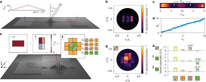
Fig. 3: Fourier pixels for amplitude, phase and polarization sensing.

Full size image

a, Schematic of a Fourier pixel that measures the phase difference \${\\varphi }\{{\\rm{in}}}\$ between light incident on two sinusoidal gratings. A central Fourier element adds a phase difference \${\\varphi }\{{\\rm{out}}}\$ between the two diffracted SPP fields that depends on the output angle \$\\theta \$ (inset). b, Optical output for \${\\varphi }\{{\\rm{in}}}=0\$, showing two dark nodes corresponding to destructive interference at specific normalized in-plane momenta \${k}\{x}/{k}\{0}\$. c, Optical output that highlights the interference minima at \${\\hat{\\varphi }}\{{\\rm{out}}}\$ used to determine the measured phase difference \${\\hat{\\varphi }}\{{\\rm{in}}}={{\\rm{\\pi }}-\\hat{\\varphi }}\{{\\rm{out}}}\$. d, Experimental calibration of the sensor relating the extracted \${\\hat{\\varphi }}\{{\\rm{in}}}\$ to the applied phase difference \${\\varphi }\{{\\rm{in}}}\$. e,f, Concept of a vectorial Fourier pixel functioning as a full Stokes sensor (amplitude and polarization). SPPs travelling along \$x\$ generate a rectangular image at the output plane with flat amplitude and no added phase (maroon rectangle). SPPs travelling along \$y\$ generate a second flat-amplitude rectangular image at the output plane with maroon, salmon, grey and light blue regions, in which the Fourier element adds \${\\varphi }\{{\\rm{out}}}\$ of \$0\$, \${\\rm{\\pi }}/2\$, \${\\rm{\\pi }}\$ and \$3{\\rm{\\pi }}/2\$, respectively. When these rectangular images are superposed, the output intensities in different regions (orange, brown and green) yield the Stokes parameters \${S}\{0}\$, \${S}\{1}\$, \${S}\{2}\$ and \${S}\_{3}\$, enabling retrieval of the total intensity and the degree of linear/circular polarization (Methods). g, Optical output for an input with diagonal linear polarization. Only the brighter orange regions (top and left) are used for analysis, as the nominally equivalent orange regions (bottom and right) exhibit slightly reduced intensity owing to fabrication imperfections. h–j, Retrieved Stokes parameters for inputs with diagonal linear (h), right circular (i) and left circular (j) polarization. The dimensions of the structures in a and e are exaggerated for clarity. The wavelength was 555 nm. Designs and SEM images for all devices are shown in Extended Data Fig. 2.

Figure 3c shows the optical output versus \${\\varphi }\{{\\rm{out}}}\$, with \${\\hat{\\varphi }}\{{\\rm{out}}}\$ marking the output phase with maximal destructive interference (at two outcoupling angles \$\\theta \$). The measured phase difference between the input beams is \${\\hat{\\varphi }}\{{\\rm{in}}}={\\rm{\\pi }}-{\\hat{\\varphi }}\{{\\rm{out}}}\$. By systematically varying the input phase difference \${\\varphi }\{{\\rm{in}}}\$ with an SLM (Methods), we retrieved \${\\hat{\\varphi }}\{{\\rm{in}}}\$ from the measured \${\\hat{\\varphi }}\_{{\\rm{out}}}\$ (Fig. 3d), finding excellent agreement. The Fourier pixel was so sensitive that it was limited by our experimental setup. Changes in the pixel output over time were consistent with fluctuations of 0.07° in the laser that launched the SPPs (Extended Data Fig. 6b). Although the sensor in Fig. 3a projects its output to the Fourier plane, we also created phase sensors with outputs in the sample plane or in an arbitrary plane (Extended Data Figs. 7a–e and 8a–c).

For polarization detection, we designed and fabricated a vectorial Fourier pixel that combines the functionalities of linear polarizers, half-wave plates and quarter-wave plates to provide a full Stokes sensor in a single thin element (Extended Data Fig. 6c). Light with unknown polarization \${{\\bf{E}}}\{{\\rm{in}}}\$ strikes two orthogonal gratings (Fig. 3e). The SPPs launched in the two paths contain information about the amount of \$x\$ and \$y\$ polarization in \${{\\bf{E}}}\{{\\rm{in}}}\$ as well as their relative phase. The Fourier element then projects two images at the output Fourier plane. SPPs travelling along \$x\$ (blue arrow) generate a flat-amplitude rectangular image with no added phase \${\\varphi }\{{\\rm{out}}}\$ (maroon rectangle, Fig. 3e), whereas SPPs travelling along \$y\$ (red arrow) generate an orthogonal flat-amplitude rectangular image subdivided into regions, in which the Fourier element adds \${\\varphi }\{{\\rm{out}}}\$ of \$0\$, \${\\rm{\\pi }}/2\$, \${\\rm{\\pi }}\$ and \$3{\\rm{\\pi }}/2\$ (maroon, salmon, grey and light blue regions, respectively, in Fig. 3e). When the two rectangles are coherently superposed in the output plane (Fig. 3f), the result is

$${{\\bf{E}}}\{{\\rm{out}}}={{\\bf{E}}}\{{\\rm{in}}}\\cdot \\hat{{\\bf{x}}}+{({\\bf{E}}}\{{\\rm{in}}}\\cdot \\hat{{\\bf{y}}}){{\\rm{e}}}^{{\\rm{i}}{\\varphi }\{{\\rm{out}}}}$$

Thus, by reading the intensity in the different regions of the output plane (Fig. 3f) with a fixed analyser, the Stokes parameters (\${S}\{0}\$, \${S}\{1}\$, \${S}\{2}\$ and \${S}\{3}\$) for the incident polarization state are retrieved (Methods). Specifically, the total input intensity (\${S}\{0}\$) is obtained by summing the orange regions, whereas the degree of linear polarization along \$x\$ or \$y\$ (\${S}\{1}\$) is their difference. The two brown central regions compare \$0\$ and \${\\rm{\\pi }}\$ phase shifts added to the \$y\$ electric field, analogous to inserting a half-wave plate. Their difference provides the degree of linear polarization along axes ±45° from \$x\$ (\${S}\{2}\$). Similarly, the difference between the two green regions, which introduce \${\\rm{\\pi }}/2\$ and \$3{\\rm{\\pi }}/2\$ phase shifts, reveals the degree of circular polarization (\${S}\{3}\$).

We tested our Stokes sensor using linearly and circularly polarized input beams. Figure 3g shows the output Fourier plane for an input beam with diagonal linear polarization (see Extended Data Fig. 6d,e for circular input polarizations). Such raw images represent the experimental version of Fig. 3f. Figure 3h–j shows the retrieved Stokes parameters for diagonal linear (\${S}\{1}=1\$), right circular (\${S}\{3}=-1\$) and left circular (\${S}\{3}=1\$) polarization: \${S}\{1}=0.87\$, \${S}\{3}=-0.83\$ and \${S}\{3}=+0.77\$, respectively. Again, although the sensor in Fig. 3e projects its output to the Fourier plane, polarization sensors with outputs in the sample plane or an arbitrary plane are shown in Extended Data Figs. 7f–j and 8d–g.

A further advantage of Fourier pixels is their ability to combine functionalities. This is missing in other methods, preventing compact single-shot characterization of complex optical fields. We demonstrate two different routes to sense amplitude, phase and polarization within a compact architecture. First, we cluster two phase sensors (for \$x\$ and \$y\$) and a Stokes sensor (Fig. 4a), exploiting three Fourier elements that project to different locations in the output Fourier plane (Fig. 4b, reconstructed from three separate measurements). Each phase sensor generates a pair of redundant interference bands (as in Fig. 3b) at the edge (top and bottom for \$x\$; left and right for \$y\$); the Stokes sensor generates an image (the same data shown in Fig. 3g) in the centre. By examining the combined output, the light striking the device can be fully analysed. In the second architecture, the three individual Fourier elements in Fig. 4a are superposed (Fig. 4c, with minor design adjustments to the Stokes sensor, and Extended Data Fig. 9a,b). Figure 4d,e shows SEMs of two examples: four gratings surround a Fourier element 30 × 30 µm2 and 10 × 10 µm2 in size, respectively. The outputs (Fig. 4f,g) again provide amplitude, phase and polarization detection but now using a footprint comparable to conventional pixels. Using the device in Fig. 4a, we mapped the phase or polarization of larger complex field profiles (Methods), including optical vortices (Fig. 4h) and trefoil aberrations (Fig. 4i), as well as polarization singularities of vector beams (Fig. 4j).

Fig. 4: Multifunctional devices for full sensing of optical fields.

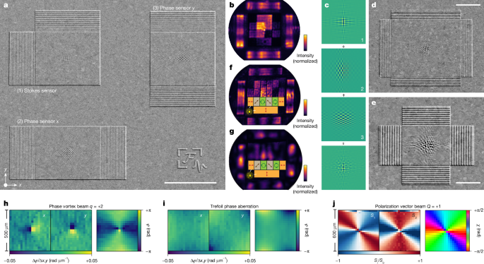
Fig. 4: Multifunctional devices for full sensing of optical fields.

Full size image

a, First design strategy for simultaneous sensing of amplitude, phase and polarization. SEM (35° tilt) of three individual sensors clustered to detect (1) amplitude and polarization; (2) phase along \$x\$; and (3) phase along \$y\$. b, Output from the device in a, constructed from three different measurements (one for each sensor to correct for microscope misalignments). The polarization sensor projects to the central region (as in Fig. 3f,g). Phase information is projected to two pairs of interference bands at the edges of Fourier space (top and bottom for \$x\$; left and right for \$y\$). c, Second design strategy for simultaneous sensing of amplitude, phase and polarization. Three Fourier elements are superposed in a single Fourier pixel. d,e, SEMs of the experimental implementation of c (35° tilt). The Fourier elements are 30 × 30 µm2 (d) and 10 × 10 µm2 (e). f,g, Output planes from the pixels in d and e, respectively, constructed from three different measurements (one for each sensor functionality). The polarization and phase sensors project as in Fig. 4b, but the polarization regions are positioned differently. Extended Data Fig. 9c–e shows single-shot measurements for the same sensors. h–j, Experimental demonstration of phase and polarization imaging with the device in a. h,i, Phase maps of a vortex beam (h; \$q=+2\$; \$\\varphi ={{\\rm{e}}}^{2{\\rm{i}}\\theta }\$) and trefoil aberrations (i; \$\\varphi ={x}^{3}-3x{y}^{2}\$) reconstructed from phase gradients along \$x\$ and \$y\$ (Methods). j, Measurement of the in-plane polarization angle \$\\chi \$ of a first-order vector beam through the Stokes parameters \${S}\{1}\$ and \${S}\{2}\$. The spatial resolution of the reconstructed maps is 25 µm, determined by the size of the Fourier pixel. The wavelengths are 562 nm in a, b and h–j and 555 nm in d–g. Scale bars, 20 μm (a), 10 μm (d), 5 μm (e), 500 μm (h), 600 μm (j).

Discussion and outlook

Because the surface profiles in our Fourier pixels are shallow, we estimate that higher-order crosstalk between functionalities is 105 times smaller than the desired outputs (Methods). Shallow profiles also allow the pixels to exploit linear diffraction theory, greatly simplifying their design. Indeed, no electromagnetic simulations were performed in this study. Typically, only 1 day is required to go from an idea to a functioning device.

Although we used gratings as SPP sources, subwavelength slits or apertures could launch SPPs in optical transmission42."). Coherent SPPs could also be generated on chip thermally11."), electrically43.") or through energy transfer from quantum emitters44."). Beyond plasmonic devices, dielectric Fourier pixels could exploit photonic waveguide modes in materials such as silicon, silicon nitride or lithium niobate. Indeed, Fig. 1h demonstrates a silicon nitride Fourier pixel that projects an image onto the Fourier plane. Such devices can be incorporated within photonic integrated circuits.

Our current sensors were designed for a specific wavelength. Spectroscopic information could be collected by clustering Fourier pixels designed for different wavelengths. Arrays of Fourier pixels could then enable ‘camera–displays’ for simultaneous detection and generation of light. Extended Data Fig. 9f shows an SEM of a small 2 × 3 array of plasmonic Fourier pixels (10 × 10 µm2 full-field sensors). Although such pixels are static, their outputs could be adjusted by the addition of tunable45."),46.") or nonlinear materials. Extended Data Fig. 10 demonstrates the potential of this approach with several examples. By varying the phase along the input gratings with an SLM, we tuned the output of the static Fourier pixel. We adjusted an output beam from linear to elliptical to circular polarization, and we moved a projected line vertically and horizontally. Finally, we created a device with bidirectional functionality. The pixel measures the phase of incident light, projecting the answer to the Fourier plane. Simultaneously, it creates a focused spot at an intermediate plane. Because the focal position depends on the input phase, the phase measurement allows prediction or correction of the focal position. With such bidirectionality, Fourier pixels provide previously unavailable functionalities and establish a universal platform for a broad class of simple-to-design modular optical devices.

Methods

Fourier-pixel design

Each Fourier pixel involves the generation, propagation and diffraction of guided waves (Fig. 1a). Although we focus here on SPPs, the design principles also apply to photonic waveguide modes. In our plasmonic Fourier pixels, we used sinusoidal gratings to generate SPPs. The SPPs were launched when the SPP wavevector, \${k}\_{{\\rm{SPP}}}\$, satisfied (Extended Data Fig. 1)

$${k}\{{\\rm{SPP}}}={k}\{\\parallel }+n{g}\_{{\\rm{m}}}$$

(1)

where \${k}\{\\parallel }\$ is the in-plane wavevector of photons incident on the grating, \${g}\{{\\rm{m}}}=2{\\rm{\\pi }}/\\varLambda \$ is the grating momentum, \$\\varLambda \$ is the grating period and \$n\$ is the diffraction order. The photons have wavevector \${\\bf{k}}\$ with \$|{\\bf{k}}|=k=\\frac{2{\\rm{\\pi }}}{\\lambda }\$ with wavelength \$\\lambda \$. If the grating contains multiple spatial frequencies, it can couple photons of different wavelengths simultaneously at the same incident angle, launching SPPs with different \${k}\_{{\\rm{SPP}}}\$.

In a Fourier pixel, the generated SPPs propagate in \$x\$ across the \$x,y\$ interfacial plane with transverse-magnetic polarization. We treat the SPPs as scalar reference waves of the form

$$r(x,y)={{\\rm{e}}}^{{\\rm{i}}{k}\_{{\\rm{SPP}}}x}$$

(2)

The SPPs then encounter the Fourier element that creates a desired complex-valued optical wavefront \$g(x,y)\$ at a specific output plane through diffraction. For simplicity, we assumed a constant-amplitude SPP wave, neglecting propagation and outscattering-induced attenuation over the extent of the Fourier element. For higher-efficiency designs, such attenuation can be compensated by apodization of the scattering strength, as commonly used in integrated photonics, guided-wave holography and metasurface systems.

The inverse-design process for our Fourier pixels must predict the height profile \${h}\_{{\\rm{p}}}(x,y)\$ of the Fourier element that generates the desired \$g(x,y)\$. In general, diffraction of light by metallic surfaces can be treated by considering the local optical path differences introduced by the structured interface. We apply a similar diffraction model to describe the interaction of SPPs with our Fourier elements. For amplitude and phase, we use a scalar diffraction model. After the SPP reference wave \$r(x,y)\$ interacts with the Fourier element, the optical wavefront at the diffractive surface, \$f(x,y)\$, is described by the relation

$$f(x,y)=r(x,y)\\,t(x,y)$$

(3)

where we introduced a complex-valued transparency function \$t(x,y)\$. It describes how the Fourier element converts the SPPs into the desired wavefront at the diffractive surface. This wavefront then propagates to generate \$g(x,y)\$. Equation (3) can be rearranged to give

$$t(x,y)=\\frac{f(x,y)}{r(x,y)}=f(x,y){{\\rm{e}}}^{-{{\\rm{i}}k}\_{{\\rm{S}}{\\rm{P}}{\\rm{P}}}x}$$

(4)

Our Fourier elements predominantly affect the local phase, \$\\phi (x,y)\$, which is a real quantity. Thus, we must consider experimentally realizable transparency functions of the form \$\\mathop{t}\\limits^{ \\sim }(x,y)={{\\rm{e}}}^{{\\rm{i}}\\phi (x,y)}\$. Further, for shallow profiles (and correspondingly small phase shifts), we can linearize the optical response as

$$\\mathop{t}\\limits^{ \\sim }(x,y)={{\\rm{e}}}^{{\\rm{i}}\\phi (x,y)}\\approx 1+{\\rm{i}}\\phi (x,y)$$

(5)

In this case, \${\\rm{I}}{\\rm{m}}\\{\\mathop{t}\\limits^{ \\sim }(x,y)\\}=\\phi (x,y)\$, which is a tuneable experimental parameter directly proportional to the local height profile, \${h}\{{\\rm{p}}}(x,y)\$. Specifically, \$\\phi (x,y)=k{h}\{{\\rm{p}}}(x,y)\$ in the limit of shallow profiles. Consequently, by adjusting \$\\phi (x,y)\$, we can set the imaginary part of the realizable transparency function \$\\mathop{t}\\limits^{ \\sim }(x,y)\$ equal to that of the desired transparency function \$t(x,y)\$ (set \${\\rm{I}}{\\rm{m}}\\{\\mathop{t}\\limits^{ \\sim }(x,y)\\}={\\rm{I}}{\\rm{m}}\\{t(x,y)\\}\$). From equation (4), we then obtain

$${\\rm{I}}{\\rm{m}}\\{\\mathop{t}\\limits^{ \\sim }(x,y)\\}=\\frac{1}{2{\\rm{i}}}\[f(x,y){{\\rm{e}}}^{-{{\\rm{i}}k}\{{\\rm{S}}{\\rm{P}}{\\rm{P}}}x}-{f}^{\\ast }(x,y){{\\rm{e}}}^{{{\\rm{i}}k}\{{\\rm{S}}{\\rm{P}}{\\rm{P}}}x}\]$$

(6)

Plugging our realizable transparency function \$\\mathop{t}\\limits^{ \\sim }(x,y)\$ into equation (3), we then obtain the realizable output \$\\mathop{f}\\limits^{ \\sim }(x,y)\$ from equations (5) and (6):

$$\\mathop{f}\\limits^{ \\sim }(x,y)=r(x,y)\\mathop{t}\\limits^{ \\sim }(x,y)={{\\rm{e}}}^{{{\\rm{i}}k}\{{\\rm{S}}{\\rm{P}}{\\rm{P}}}x}\\left\\{1+\\frac{1}{2}\[f(x,y){{\\rm{e}}}^{-{{\\rm{i}}k}\{{\\rm{S}}{\\rm{P}}{\\rm{P}}}x}-{f}^{\\ast }(x,y){{\\rm{e}}}^{{{\\rm{i}}k}\_{{\\rm{S}}{\\rm{P}}{\\rm{P}}}x}\]\\right\\}$$

(7)

$$\\mathop{f}\\limits^{ \\sim }(x,y)={{\\rm{e}}}^{{{\\rm{i}}k}\{{\\rm{S}}{\\rm{P}}{\\rm{P}}}x}+\\frac{1}{2}\[f(x,y)-{f}^{\\ast }(x,y){{\\rm{e}}}^{{2{\\rm{i}}k}\{{\\rm{S}}{\\rm{P}}{\\rm{P}}}x}\]$$

(8)

The realizable output in equation (8) contains three terms: the desired output \$f(x,y)\$ and two SPP terms. Only the term corresponding to \$f(x,y)\$ produces a wavefront that radiates into free space. The other two terms remain guided SPP modes. However, these modes do not necessarily represent dissipative loss channels. In Fourier pixels, the SPPs propagate in-plane and continuously interact with the Fourier element. Energy can therefore be continuously scattered from the guided mode into free space. These non-radiative SPP components thus act as intermediate guided fields.

Equation (8) states that the realizable Fourier element can create any desired \$f(x,y)\$. If the required \$f(x,y)\$ is known, the necessary height profile can be determined from equation (6) in the limit of shallow profiles:

$${h}\{{\\rm{p}}}(x,y)=\\frac{1}{2{\\rm{i}}k}\[f(x,y){{\\rm{e}}}^{-{{\\rm{i}}k}\{{\\rm{S}}{\\rm{P}}{\\rm{P}}}x}-{f}^{\\ast }(x,y){{\\rm{e}}}^{{{\\rm{i}}k}\_{{\\rm{S}}{\\rm{P}}{\\rm{P}}}x}\]$$

(9)

The inverse-design process now involves predicting the complex-valued optical wavefront \$f(x,y)\$ at the sample plane (at \$z=0\$) that leads to the desired output \$g(x,y)\$. For outputs at arbitrary planes (\$z=d\$), we used the Fresnel approximation. For outputs in the far field (or in our case at \$z=2{f}\{{\\ell }}\$, the back focal plane of a lens with focal length \${f}\{{\\ell }}\$), we used the Fraunhofer approximation. The desired output \$g(x,y)\$ was backpropagated through the angular spectrum method or the inverse Fourier transform, respectively, to obtain the corresponding complex-valued wavefront \$f(x,y)\$ at the sample plane. In the Fresnel regime, this gives a convolution integral over positional coordinates \$(\\xi ,\\eta )\$

$$f(x,y)={\\iint }\_{-{\\rm{\\infty }}}^{{\\rm{\\infty }}}g(\\xi ,\\eta )h(x-\\xi ,y-\\eta ,-d){\\rm{d}}\\xi {\\rm{d}}\\eta $$

(10)

where the convolution kernel \$h(x,y,z)\$ is the Fresnel impulse response

$$h(x,y,d)=\\frac{{{\\rm{e}}}^{{\\rm{i}}kd}}{{\\rm{i}}\\,\\lambda \\,d}\\,\\exp \\,\\left\[\\frac{{\\rm{i}}\\,\\pi }{\\lambda \\,d}({x}^{2}+{y}^{2})\\right\]$$

(11)

In the Fraunhofer regime, \$g(x,y)\$ can be represented as a function of spatial frequencies \${k}\{x}\$ and \${k}\{y}\$:

$$\\mathop{g}\\limits^{ \\sim }({k}\{x},{k}\{y}):= g\\left(x=\\frac{{k}\{x}\\,{f}\{{\\ell }}}{k},y=\\frac{{k}\{y}\\,{f}\{{\\ell }}}{k}\\right)$$

(12)

leading to

$$f(x,y)={\\rm{i}}\\,\\lambda \\,{f}\{{\\ell }}\\,\\exp (-{\\rm{i}}2k{f}\{{\\ell }})\\,{{\\mathcal{F}}}^{-1}\\{\\mathop{g}\\limits^{ \\sim }({k}\{x},{k}\{y})\\}$$

(13)

$$f(x,y)=\\frac{{\\rm{i}}\\,\\lambda \\,{f}\{{\\ell }}}{4\\,{\\pi }^{2}}\\,\\exp (-{\\rm{i}}2k{f}\{{\\ell }})\\,{\\iint }\{-{\\rm{\\infty }}}^{{\\rm{\\infty }}}\\mathop{g}\\limits^{ \\sim }({k}\{x},{k}\{y})\\exp \[{\\rm{i}}({k}\{x}\\,x+{k}\{y}\\,y)\]{\\rm{d}}{k}\{x}{\\rm{d}}{k}\_{y}$$

(14)

With the formulas for \$f(x,y)\$ (equations (10) or (14)), we can then determine the required height profile for the Fourier element using equation (9).

The above scalar diffraction model can be generalized to include polarization and treat vectorial Fourier pixels. SPPs are coherently launched along two perpendicular directions \$x\$ and \$y\$. We define two-dimensional vectors for the desired optical output \${\\bf{g}}(x,y)\$, the backpropagated counterpart \${\\bf{f}}(x,y)\$ and the reference waves \${\\bf{r}}(x,y)\$:

$${\\bf{g}}(x,y)=\\left\[\\begin{array}{c}{g}\{x}(x,y)\\\\ {g}\{y}(x,y)\\end{array}\\right\],\\,{\\bf{f}}(x,y)=\\left\[\\begin{array}{c}{f}\{x}(x,y)\\\\ {f}\{y}(x,y)\\end{array}\\right\],\\,{\\bf{r}}(x,y)=\\left\[\\begin{array}{c}{{\\rm{e}}}^{{{\\rm{i}}k}\{{\\rm{S}}{\\rm{P}}{\\rm{P}}}x}\\\\ {{\\rm{e}}}^{{{\\rm{i}}k}\{{\\rm{S}}{\\rm{P}}{\\rm{P}}}y}\\end{array}\\right\]$$

(15)

The realizable system response is described by the transparency matrix

$$\\mathop{T}\\limits^{ \\sim }(x,y)=\\left\[\\begin{array}{cc}\\mathop{t}\\limits^{ \\sim }(x,y) & 0\\\\ 0 & \\mathop{t}\\limits^{ \\sim }(x,y)\\end{array}\\right\]$$

(16)

with

$$\\begin{array}{l}\\mathop{t}\\limits^{ \\sim }(x,y)=1+\\frac{1}{2}\[{f}\{x}(x,y){{\\rm{e}}}^{-{{\\rm{i}}k}\{{\\rm{S}}{\\rm{P}}{\\rm{P}}}x}-{f}\{x}^{\\ast }(x,y){{\\rm{e}}}^{{{\\rm{i}}k}\{{\\rm{S}}{\\rm{P}}{\\rm{P}}}x}\\\\ \\,+\\,{f}\{y}(x,y){{\\rm{e}}}^{-{{\\rm{i}}k}\{{\\rm{S}}{\\rm{P}}{\\rm{P}}}y}-{f}\{y}^{\\ast }(x,y){{\\rm{e}}}^{{{\\rm{i}}k}\{{\\rm{S}}{\\rm{P}}{\\rm{P}}}y}\]\\end{array}$$

(17)

and

$$\\begin{array}{c}{h}\{{\\rm{p}}}(x,y)=\\frac{1}{2{\\rm{i}}k}\[{f}\{x}(x,y){{\\rm{e}}}^{{-{\\rm{i}}k}\{{\\rm{S}}{\\rm{P}}{\\rm{P}}}x}-{f}\{x}^{\\ast }(x,y){{\\rm{e}}}^{{{\\rm{i}}k}\{{\\rm{S}}{\\rm{P}}{\\rm{P}}}x}\\\\ \\,+\\,{f}\{y}(x,y){{\\rm{e}}}^{{-{\\rm{i}}k}\{{\\rm{S}}{\\rm{P}}{\\rm{P}}}y}-{f}\{y}^{\\ast }(x,y){{\\rm{e}}}^{{{\\rm{i}}k}\_{{\\rm{S}}{\\rm{P}}{\\rm{P}}}y}\],\\end{array}$$

(18)

in the limit of shallow profiles. The realizable response at the sample plane is given by \$\\mathop{{\\bf{f}}}\\limits^{ \\sim }(x,y)=\\mathop{T}\\limits^{ \\sim }(x,y){\\bf{r}}(x,y)\$. Each polarization component contributes five distinct terms. As in equation (8), only the term containing the desired wavefront couples to free space.

Efficiency of Fourier pixels

The efficiency of Fourier pixels was estimated using focusing pixels (similar to that in Fig. 1i). The optical power that was focused to the desired spot \${I}\{{\\rm{focus}}}\$ was compared with the total power \${I}\{{\\rm{tot}}}\$ incident on the input grating. An excitation mask selectively illuminated the grating region under oblique incidence, launching SPPs selectively in the direction of the Fourier element. We note that the incoupling gratings act as directional couplers. Efficient excitation of SPPs occurs only when the in-plane momentum of the incident light satisfies the momentum-matching condition \${k}\{\\mathrm{SPP}}={k}\{0}\\sin {\\theta }\{\\mathrm{in}}\\pm 2{\\rm{\\pi }}/\\varLambda \$. All Fourier pixels are designed for illumination close to surface-normal incidence (\${\\theta }\{{\\rm{in}}}\\,\\approx \$ 0), such that the coupling condition is fulfilled by an appropriate choice of the grating pitch \$\\varLambda \$. As a result, the reported efficiencies correspond to specific illumination geometries.

The Fourier pixel chosen for efficiency measurements was designed to act as a sinusoidal Fresnel lens. The height profile followed the function

$${h}\{{\\rm{p}}}(x,y)=A\\,\\left\\{1-\\exp \\,\\left\[-\\alpha \\,\\left(x+\\frac{L}{2}\\right)\\right\]\\right\\}\\,\\cos \\,\\left\[\\frac{\\pi ({x}^{2}+{y}^{2})}{{f}\{{\\ell }}\\lambda }-{k}\_{{\\rm{S}}{\\rm{P}}{\\rm{P}}}\\,x\\right\],$$

(19)

where \$A\$ is the height amplitude and \$L\$ is the side length of the Fourier element in \$(x,y)\$. The centre of the profile was at \$(\\mathrm{0,0})\$. To suppress back reflection and outscattering of the SPPs at the boundary between the grating and the Fourier element, equation (19) includes apodization with \$\\alpha ={k}\{{\\rm{SPP}}}/5\$. The total incident intensity \${I}\{{\\rm{tot}}}\$ was obtained from a reflection measurement from flat Ag, whereas the reflected intensity from the grating \${I}\{{\\rm{grating}}}\$ gave the incoupling efficiency \${\\eta }\{{\\rm{in}}}=1-{I}\{{\\rm{grating}}}/{I}\{{\\rm{tot}}}\$. The overall efficiency was determined from the integrated focused intensity at 25 µm above the surface as \${\\eta }\{{\\rm{tot}}}={I}\{{\\rm{focus}}}/{I}\{{\\rm{tot}}}\$. For blue (\$\\lambda \\,=\$ 450 nm; grating amplitude \$A\\,=\$ 20 nm), green (520 nm; \$A\\,=\$ 25 nm) and red (630 nm; \$A\\,=\$ 30 nm) light, the efficiencies \$\\{{\\eta }\{{\\rm{in}}},{\\eta }\_{{\\rm{tot}}}\\}\$ were \$\\{76.7 \\% ,23.8 \\% \\}\$, \$\\{72.6 \\% ,42.2 \\% \\}\$ and \$\\{70.2 \\% ,41.4 \\% \\}\$, respectively. The efficiency for 450-nm light was lower owing to increased plasmonic losses in Ag at shorter wavelengths.

To evaluate the effect of superposing multiple grating harmonics within a single incoupler, we fabricated a composite grating containing spatial frequencies for blue, green and red coupling under normal incidence. The corresponding modulation amplitudes were \$A\\,=\$ 20 nm, 25 nm and 30 nm, respectively. The measured incoupling efficiencies for the combined structure were 32.0% (blue), 50.2% (green) and 38.0% (red). Compared with single-harmonic gratings, the reduced efficiencies are attributed to the introduction of more diffraction and SPP outscattering channels arising from the superposition of multiple periodicities.

Stokes polarimetry

Arbitrary incoming light fields can be separated into their polarization components

$${A}\{x}={a}\{x}{{\\rm{e}}}^{{\\rm{i}}{\\varphi }\{x}},{A}\{y}={a}\{y}{{\\rm{e}}}^{{\\rm{i}}{\\varphi }\{y}},$$

(20)

where \$a\$ and \$\\varphi \$ are amplitude and phase, respectively. The Stokes parameters describe the polarization state of light, defined by

$${S}\{0}={|{A}\{x}|}^{2}+{|{A}\{y}|}^{2}={a}\{x}^{2}+{a}\_{y}^{2},$$

(21)

$${S}\{1}={|{A}\{x}|}^{2}-{|{A}\{y}|}^{2}={a}\{x}^{2}-{a}\_{y}^{2},$$

(22)

$${S}\{2}=2\\mathrm{Re}\\{{A}\{x}^{\* }{A}\{y}\\}=2{a}\{x}{a}\{y}\\cos ({\\varphi }\{y}-{\\varphi }\_{x}),$$

(23)

$${S}\{3}=2{\\rm{Im}}\\{{A}\{x}^{\* }{A}\{y}\\}=2{a}\{x}{a}\{y}\\sin ({\\varphi }\{y}-{\\varphi }\_{x})$$

(24)

We assumed a uniform polarization state over the Fourier-pixel area. For detection, we used a linear polarizer along the diagonal, 45° from both \$x\$ and \$y\$ axes. We measured the intensities in Fourier space corresponding to the isolated \$x\$ and \$y\$ components of the incident field, that is, \${I}\{x,y}={a}\{x,y}^{2}/2\$. From these quantities, we retrieved the first two Stokes parameters,

$${S}\{0}=2({I}\{x}+{I}\_{y}),$$

(25)

$${S}\{1}=2({I}\{x}-{I}\_{y})$$

(26)

For the other two Stokes parameters, we recombined the incoupled light fields with tailored phase shifts \${\\varphi }\_{{\\rm{out}}}\$ between the \$x\$ and \$y\$ directions. In general, the total intensity becomes

$$I({\\varphi }\{{\\rm{out}}})=\\frac{1}{2}{|{A}\{x}+{A}\{y}{{\\rm{e}}}^{{\\rm{i}}{\\varphi }\{{\\rm{out}}}}|}^{2}$$

(27)

By choosing the phases \${\\varphi }\_{{\\rm{out}}}=\\{0,{\\rm{\\pi }}/2,{\\rm{\\pi }},3{\\rm{\\pi }}/2\\}\$, we isolated the remaining Stokes parameters,

$${S}\_{2}=I(0)-I({\\rm{\\pi }}),$$

(28)

$${S}\_{3}=I(3{\\rm{\\pi }}/2)-I({\\rm{\\pi }}/2)$$

(29)

Extracting large phase profiles from phase-gradient maps

The phase profile \$\\varphi \$ was reconstructed from discrete phase-step maps \${m}\{x}\$ and \${m}\{y}\$, which represent the local-phase differences between adjacent sampling points. To recover a globally consistent phase, a self-consistency equation between the phase profile and its gradients was solved:

$${\\nabla }^{2}\\varphi =\\frac{\\partial {m}\{x}}{\\partial x}+\\frac{\\partial {m}\{y}}{\\partial y}:= M$$

(30)

where the middle of equation (30) was obtained from finite differences of the measured phase-step maps. This self-consistency procedure avoids the accumulation of noise that occurs when the phase is retrieved by direct integration. The equation was converted to the spatial-frequency domain using a two-dimensional fast Fourier transform (2D FFT). In the discrete Fourier domain (denoted by the ^ symbol), the solution is

$$\\hat{\\varphi }=\\frac{\\hat{M}}{2\\cos ({k}\{x})+2\\cos ({k}\{y})-4},$$

(31)

with the zero-frequency component set to zero to fix the arbitrary phase offset. An inverse 2D FFT then yielded the phase profile \$\\varphi \$.

Fabrication of plasmonic Fourier pixels

Plasmonic Fourier pixels were fabricated using thermal scanning probe lithography (TSPL)16."). Poly(phthalaldehyde) (PPA) was used as the thermally sensitive resist. Si (100) wafers (2-in. diameter; 1-mm thickness; Silicon Materials) were first cleaned with oxygen plasma (GIGAbatch; PVA TePla) at 600 W for 2 min. Subsequently, 400 μl of a 12 wt% solution of PPA (Allresist) in anisole (AR 600-02; Allresist) was spin-coated onto the wafers using a two-step procedure: (1) 5 s at 500 rpm with a ramp of 500 rpm s−1; and (2) 40 s at 2,000 rpm with 2,000 rpm s−1. After baking the PPA layer on a hot plate at 110 °C for 2 min, a uniform film thickness of 350–400 nm was obtained. To pattern the PPA, the Fourier-pixel height profiles were loaded into the TSPL tool (NanoFrazor Explore; Heidelberg Instruments) as 8-bit bitmaps (256 depth levels in \$z\$ for each 20 × 20 nm2 region in \$x,y\$; ref. 16.")). In practice, owing to the tip shape, heat transfer, material flow and so on, continuous surface profiles were obtained at our length scales. Specific parameters (depth range, writing time per pixel and feedback gains) were adjusted depending on the design. The writing depth was controlled through electrostatic actuation between the cantilever and substrate. For feedback during writing, the TSPL tool used in situ topography data.

To replicate the obtained pattern in a plasmonic material, a layer of Ag more than 600 nm thick was deposited onto the patterned PPA by thermal evaporation (NANO 36; Kurt J. Lesker) using Ag pellets (99.999%; 1/4-in. diameter × 1/4-in. length; Kurt J. Lesker). The deposition rate was maintained at 2.5 nm s−1 under high vacuum (3 × 10−7 mbar)39."). Subsequently, we attached a 1-mm-thick glass slide (Paul Marienfeld) on top of the Ag surface using ultraviolet-curable epoxy (OG142-95; Epoxy Technology). The glass slide was allowed to rest on the epoxy for 5 min before exposure to ultraviolet light (2 h), which minimized PPA contamination on the Ag. The cured glass/epoxy/Ag stack was stripped from the PPA substrate using a razor blade13."), revealing the surface structure in Ag (inverted from the original PPA pattern). A final cleaning step in anisole (AR 600-02; Allresist) for 2 min removed any residual PPA from the Ag.

Fabrication of dielectric Fourier pixels

Dielectric Fourier pixels were fabricated on Si substrates coated with dielectric thin films. Si (100) wafers (525-μm thickness; Si-Mat Silicon Materials) were first thermally oxidized to form a 2.85-µm SiO2 layer (TS3604; Tempress), followed by deposition of a 225-nm high-stress SiN_x_ film by low-pressure chemical vapour deposition. For the low-pressure chemical vapour deposition process, dichlorosilane (70 sccm) and NH3 (210 sccm) were used as precursor gases at 800 °C and 200 mTorr. The wafers were then diced into 15 × 15 mm2 chips. Before resist coating, the chips were cleaned in acetone for 2 min, isopropanol for 2 min and oxygen plasma for 5 min at 600 W. A 12 wt% solution of PPA was spin-coated in a single step at 6,000 rpm, resulting in a resist thickness of 258 nm. Greyscale Fourier-pixel patterns were subsequently written into the PPA using TSPL. The pattern was then transferred into the SiN_x_ layer by reactive ion etching (PlasmaPro NPG 80, Oxford Instruments) using CHF3 (50 sccm) and O2 (5 sccm) at 100 W. The selectivity for etching was 1.4. After etching, the chips were cleaned again in acetone for 2 min, isopropanol for 2 min and oxygen plasma for 5 min at 600 W.

Design parameters

The sinusoidal grating pitch, \$\\varLambda \$, was 509 nm for all Fourier pixels in this study, except those in Fig. 1h (353 nm) and Extended Data Figs. 4h (417 nm, 509 nm and 618 nm) and 7b,g (495 nm). The sinusoidal grating amplitude, A, was 25 nm for all Fourier pixels, except for those in Fig. 1h (23 nm) and Extended Data Fig. 4h (20 nm, 25 nm and 30 nm). The depth, \${h}\_{{\\rm{p}}}\$, of the Fourier element was 50 nm for the pixels in Fig. 1i,j and Extended Data Figs. 5, 7, 8 and 10h; 140 nm for the pixel in Fig. 1h; 150 nm for the pixels in Figs. 1d–g, 2c,d, 3b,g and 4a,d,e and Extended Data Figs. 4a–g, 9c–f and 10a; 200 nm for the pixel in Extended Data Fig. 10j; and 250 nm for the pixels in Fig. 2e,f and Extended Data Fig. 4h.

Optical measurements

The optical setup is depicted in Extended Data Fig. 3. Fourier pixels were measured using a home-built optical apparatus based on an inverted optical microscope (Eclipse Ti-U; Nikon) equipped with a 50× air objective (TU Plan Fluor; Nikon; numerical aperture of 0.8). A filtered (LLTF Contrast; NKT Photonics; 420–1,000-nm accessible wavelengths; linewidth of approximately 1.5 nm) supercontinuum laser (SuperK FIU−15; NKT Photonics) allowed illumination of the sample at different wavelengths. After passing through a short-pass optical filter (FESH0750; Thorlabs), the laser beam was then collimated with a 10× objective (L1; TU Plan Fluor; Nikon; numerical aperture of 0.3). This objective was used to reduce chromatic aberrations, which could cause a spread of incoming angles at the sample. The collimated beam was focused onto the back focal plane of the microscope objective by a 400-mm defocusing lens (L2), resulting in a 100× demagnified Gaussian illumination spot on the sample. Laser-cut cardboard masks (Extended Data Fig. 3d) were placed in the excitation path to selectively illuminate the incoupling gratings. A rotatable linear polarizer in the excitation path controlled SPP launching from the two orthogonal incoupling gratings (Fig. 2a). More specifically, SPP launching was maximized for one grating by aligning the incoming polarization with its corrugations or evenly divided over two orthogonal gratings by orienting the polarization at 45° between them. Diffracted light off the substrate was passed through a circular aperture in the image plane to isolate light emanating from the Fourier element. For all Fourier pixels designed to project the output to the far field (Extended Data Fig. 3a), the back focal plane of the microscope objective was imaged on a digital camera (Zyla PLUS sCMOS; Andor). For Fourier pixels that project to arbitrary planes (Extended Data Fig. 3b), lens L6 was removed to image the sample plane or a plane displaced along the optical axis, selected by moving the microscope turret relative to the sample.

For measurements with incoherent illumination (Extended Data Fig. 4g), the laser source was replaced by a halogen lamp spectrally filtered with a 10-nm full-width-at-half-maximum bandpass filter. The angular spectrum of the lamp was further restricted by placing a mask in a Fourier plane in the excitation path, ensuring SPP launching into a single direction.

To control the phase of the incoming laser, a liquid-crystal spatial light modulator (SLM; PLUTO NIR011; HOLOEYE) was used (Extended Data Fig. 3c). The SLM display was imaged onto the Fourier pixel by replacing L2 with a 750-mm lens (instead of the 400-mm lens). With the microscope objective, this resulted in a demagnification of 187.5×. The SLM display was subdivided into two regions, and the relative phase between them was systematically varied between \$0\$ and \$2{\\rm{\\pi }}\$. The two incoupling gratings (Fig. 3a and Extended Data Fig. 10) were illuminated by the two regions of the SLM, thereby tuning the incoming phase difference. This measurement procedure was also used to systematically project parts of large complex phase profiles onto the phase sensors of the Fourier pixel (Fig. 4h,i).

To systematically control the in-plane polarization of the incoming laser (Fig. 4j), a rotatable mechanical mount (PRM1Z8; Thorlabs) was used in combination with a linear polarizer and custom-built control software. This configuration provided adjustable linear polarization, as the laser source is unpolarized in-plane. A quarter-wave plate was used together with the linear polarizer, oriented at −45° or +45°, to generate left or right circularly polarized light (Fig. 3i,j), respectively. In the detection path, a linear polarizer projected the diffracted light onto the axis at 45° between the gratings to extract the Stokes parameters.

Potential for unwanted crosstalk in multifunctional Fourier pixels

When multiple diffractive surface profiles are superposed in a Fourier pixel, one must consider the possibility of crosstalk. In principle, superposition of spatial frequencies in the Fourier element can generate undesired mixed diffraction orders. To address this possibility, we performed a quantitative analysis of the expected crosstalk based on the spatial frequency content of our diffractive Fourier elements. Taking the Fourier pixel in Extended Data Fig. 2a,b as an example, which has a maximum modulation depth of \${h}\_{{\\rm{p}}}=\$ 150 nm, we determined the contribution of individual spatial frequencies by computing the 2D FFT. After normalization to the physical height modulation, we found an effective depth per spatial frequency component of approximately 0.5 nm, indicating that the total surface relief is distributed across many spatial frequencies.

To estimate the crosstalk, we consider a simple scalar diffraction model consisting of two sinusoidal gratings with spatial frequencies \${g}\{1}\$ and \${g}\{2}\$ and depth \$h\$ equal to the depth extracted above. Superposition can generate undesired higher-order contributions, such as \${g}\{1}+{g}\{2}\$. The diffraction efficiencies \${\\eta }\{m,n}\$ of the different orders \${{mg}}\{1}+n{g}\_{2}\$, where \$m\$ and \$n\$ are integers, can be found from

$${\\eta }\{m,n}\\propto {J}\{m}{({kh})}^{2}{J}\_{n}{({kh})}^{2}$$

(32)

where \$k\$ is the free-space wavevector, and \${J}\{i}\$ is the Bessel function of the first kind of order \$i\$. We defined the desired first-order efficiency as \${\\eta }\{\\mathrm{1,0}}\$ and the mixed-order efficiency as \${\\eta }\{\\mathrm{1,1}}\$. We then calculated the resulting efficiency ratio \${\\eta }\{\\mathrm{1,0}}/{\\eta }\_{\\mathrm{1,1}}\$ as a function of modulation depth in the pattern. For the depth extracted from the Fourier element (\$h\\,\\approx \$ 0.5 nm), the ratio exceeded 105, indicating that crosstalk is more than five orders of magnitude weaker than the desired diffraction process.

The above argument relies on the fact that the Fourier element contains many spatial frequencies, which is the case for all of the devices in this study. If a structure (for example, a sinusoidal grating) had only a handful of spatial frequencies, crosstalk could become more important.

In addition, using guided surface modes as the reference wave further suppresses undesired diffraction losses. The momentum of these guided waves lies outside the free-space light cone, whereas the desired optical output is typically near the surface normal. As a result, diffraction from a single spatial frequency produces only one propagating free-space order; other orders remain evanescent and do not contribute an optical signal.

Data availability

Data supporting the findings of this study can be obtained from the corresponding author upon request.

References

1. Janesick, J. R., Elliott, T., Collins, S., Blouke, M. M. & Freeman, J. Scientific charge-coupled devices. Opt. Eng. 26, 692–714 (1987). ADS CAS Google Scholar 2. Huang, Y., Hsiang, E.-L., Deng, M.-Y. & Wu, S.-T. Mini-LED, micro-LED and OLED displays: present status and future perspectives. Light: Sci. Appl. 9, 105 (2020). Article ADS CAS PubMed PubMed Central Google Scholar 3. Lyon, R. A brief history of ‘pixel’. Proc. SPIE 6069, 606901 (2006). Article Google Scholar 4. Oh, N. et al. Double-heterojunction nanorod light-responsive LEDs for display applications. Science 355, 616–619 (2017). Article ADS CAS PubMed Google Scholar 5. Bao, C. et al. A multifunctional display based on photo-responsive perovskite light-emitting diodes. Nat. Electron. 7, 375–382 (2024). Article CAS Google Scholar 6. Tittl, A. et al. Imaging-based molecular barcoding with pixelated dielectric metasurfaces. Science 360, 1105–1109 (2018). Article ADS MathSciNet CAS PubMed Google Scholar 7. Tang, X., Ackerman, M. M., Chen, M. & Guyot-Sionnest, P. Dual-band infrared imaging using stacked colloidal quantum dot photodiodes. Nat. Photonics 13, 277–282 (2019). Article ADS CAS Google Scholar 8. Yang, Z. et al. Single-nanowire spectrometers. Science 365, 1017–1020 (2019). Article ADS CAS PubMed Google Scholar 9. Goodman, J. W. Introduction to Fourier Optics (W. H. Freeman,2017). Google Scholar 10. Barnes, W. L., Dereux, A. & Ebbesen, T. W. Surface plasmon subwavelength optics. Nature 424, 824–830 (2003). Article ADS CAS PubMed Google Scholar 11. Greffet, J. J. et al. Coherent emission of light by thermal sources. Nature 416, 61–64 (2002). Article ADS CAS PubMed Google Scholar 12. Gorodetski, Y., Niv, A., Kleiner, V. & Hasman, E. Observation of the spin-based plasmonic effect in nanoscale structures. Phys. Rev. Lett. 101, 043903 (2008). Article ADS CAS PubMed Google Scholar 13. Nagpal, P., Lindquist, N. C., Oh, S.-H. & Norris, D. J. Ultrasmooth patterned metals for plasmonics and metamaterials. Science 325, 594–597 (2009). Article ADS CAS PubMed Google Scholar 14. Spektor, G. et al. Revealing the subfemtosecond dynamics of orbital angular momentum in nanoplasmonic vortices. Science 355, 1187–1191 (2017). Article ADS CAS PubMed Google Scholar 15. Tsesses, S. et al. Four-dimensional conserved topological charge vectors in plasmonic quasicrystals. Science 387, 644–648 (2025). Article ADS MathSciNet CAS PubMed Google Scholar 16. Lassaline, N. et al. Optical Fourier surfaces. Nature 582, 506–510 (2020). Article ADS CAS PubMed PubMed Central Google Scholar 17. Booth, M. J. Adaptive optical microscopy: the ongoing quest for a perfect image. Light: Sci. Appl. 3, e165 (2014). Article ADS Google Scholar 18. Salter, P. S. & Booth, M. J. Adaptive optics in laser processing. Light: Sci. Appl. 8, 110 (2019). Article ADS PubMed PubMed Central Google Scholar 19. Ozaki, M., Kato, J.-I. & Kawata, S. Surface-plasmon holography with white-light illumination. Science 332, 218–220 (2011). Article ADS CAS PubMed Google Scholar 20. Gopakumar, M. et al. Full-colour 3D holographic augmented-reality displays with metasurface waveguides. Nature 629, 791–797 (2024). Article ADS CAS PubMed PubMed Central Google Scholar 21. Meng, W. et al. Ultranarrow-linewidth wavelength-vortex metasurface holography. Sci. Adv. 11, eadt9159 (2025). Article ADS CAS PubMed PubMed Central Google Scholar 22. Bütow, J., Eismann, J. S., Sharma, V., Brandmüller, D. & Banzer, P. Generating free-space structured light with programmable integrated photonics. Nat. Photonics 18, 243–249 (2024). Article ADS Google Scholar 23. Zhou, X., Yi, D., Chan, D. W. U. & Tsang, H. K. Silicon photonics for high-speed communications and photonic signal processing. npj Nanophoton. 1, 27 (2024). Article Google Scholar 24. Yousef, K. M. A. et al. Metasurface quantum graphs for generalized Hong–Ou–Mandel interference. Science 389, 416–422 (2025). Article ADS MathSciNet CAS PubMed Google Scholar 25. Casasent, D. Spatial light modulators. Proc. IEEE 65, 143–157 (1977). Article ADS CAS Google Scholar 26. Yu, N. F. & Capasso, F. Flat optics with designer metasurfaces. Nat. Mater. 13, 139–150 (2014). Article CAS PubMed Google Scholar 27. Rubin, N. A. et al. Matrix Fourier optics enables a compact full-Stokes polarization camera. Science 365, eaax1839 (2019). Article ADS CAS PubMed Google Scholar 28. Go, G.-H. et al. Meta Shack–Hartmann wavefront sensor with large sampling density and large angular field of view: phase imaging of complex objects. Light: Sci. Appl. 13, 187 (2024). Article ADS CAS PubMed PubMed Central Google Scholar 29. Li, S.-Q. et al. Phase-only transmissive spatial light modulator based on tunable dielectric metasurface. Science 364, 1087–1090 (2019). Article ADS CAS PubMed Google Scholar 30. Moitra, P. et al. Electrically tunable reflective metasurfaces with continuous and full-phase modulation for high-efficiency wavefront control at visible frequencies. ACS Nano 17, 16952–16959 (2023). Article ADS CAS PubMed Google Scholar 31. Yu, N. et al. Light propagation with phase discontinuities: generalized laws of reflection and refraction. Science 334, 333–337 (2011). Article ADS CAS PubMed Google Scholar 32. Fang, X., Ren, H. & Gu, M. Orbital angular momentum holography for high-security encryption. Nat. Photonics 14, 102–108 (2020). Article ADS CAS Google Scholar 33. Song, Q. et al. Broadband decoupling of intensity and polarization with vectorial Fourier metasurfaces. Nat. Commun. 12, 3631 (2021). Article ADS CAS PubMed PubMed Central Google Scholar 34. Overvig, A. & Alù, A. Diffractive nonlocal metasurfaces. Laser Photonics Rev. 16, 2100633 (2022). Article ADS Google Scholar 35. Shastri, K. & Monticone, F. Nonlocal flat optics. Nat. Photonics 17, 36–47 (2023). Article ADS CAS Google Scholar 36. Huang, H. et al. Leaky-wave metasurfaces for integrated photonics. Nat. Nanotechnol. 18, 580–588 (2023). Article ADS CAS PubMed Google Scholar 37. Zeng, Y. et al. Metalasers with arbitrarily shaped wavefront. Nature 643, 1240–1245 (2025). Article ADS CAS PubMed Google Scholar 38. Hen, L., Yosef, E., Raviv, D., Giryes, R. & Scheuer, J. Inverse design of diffractive metasurfaces using diffusion models. ACS Photonics 13, 38–46 (2026). Article CAS Google Scholar 39. McPeak, K. M. et al. Plasmonic films can easily be better: rules and recipes. ACS Photonics 2, 326–333 (2015). Article CAS PubMed PubMed Central Google Scholar 40. Nye, J. F. & Berry, M. V. Dislocations in wave trains. Proc. R. Soc. Lond. A 336, 165–190 (1974). Article ADS MathSciNet Google Scholar 41. Keitel, R. C. et al. Single-pulse measurement of orbital angular momentum generated by microring lasers. ACS Nano 15, 19185–19193 (2021). Article CAS PubMed Google Scholar 42. Lalanne, P., Hugonin, J. P. & Rodier, J. C. Theory of surface plasmon generation at nanoslit apertures. Phys. Rev. Lett. 95, 263902 (2005). Article ADS CAS PubMed Google Scholar 43. Du, W., Wang, T., Chu, H.-S. & Nijhuis, C. A. Highly efficient on-chip direct electronic–plasmonic transducers. Nat. Photonics 11, 623–627 (2017). Article ADS CAS Google Scholar 44. Kress, S. J. P. et al. Wedge waveguides and resonators for quantum plasmonics. Nano Lett. 15, 6267–6275 (2015). Article ADS CAS PubMed PubMed Central Google Scholar 45. Selvin, S. P. et al. Acoustic wave modulation of gap plasmon cavities. Science 389, 516–520 (2025). Article ADS CAS PubMed Google Scholar 46. Liu, W., Xu, S. & Lee, C. Ultracompact on-chip spectral shaping using pixelated nano-opto-electro-mechanical gratings. Science 389, 806–810 (2025). Article ADS CAS PubMed Google Scholar

Download references

Acknowledgements

We thank R. Keitel and L. Novotny for stimulating discussions and U. Drechsler and M. Stiefel for technical support.

Funding

Support for the research in this study was provided by the Swiss National Science Foundation (SNSF) (grant no. 2000-1-240090) to Y.M.G., D.B.S., H.N. and D.J.N. Support for the research in this study was provided by SNSF (grant no. 200021-232257) to S.J.W.V., DAAD: German Academic Exchange Service to M.F.B., SNSF (Postdoc Mobility P500PT\_211105) to N.L. and the Villum Foundation (Villum Experiment 50355) to N.L. B.d.J., E.B., D.P. and G.N. received no specific funding for this work.

Author information

Author notes 1. These authors contributed equally: Yannik M. Glauser, Sander J. W. Vonk

Authors and Affiliations

1. Optical Materials Engineering Laboratory, Department of Mechanical and Process Engineering, ETH Zurich, Zurich, Switzerland Yannik M. Glauser, Sander J. W. Vonk, David B. Seda, Hannah Niese, Boris de Jong, Matthieu F. Bidaut, Erwan Bossavit, Daniel Petter, Gabriel Nagamine, Nolan Lassaline & David J. Norris 2. Institute of Applied Physics, University of Bern, Bern, Switzerland Gabriel Nagamine 3. Department of Physics, Technical University of Denmark, Kongens Lyngby, Denmark Nolan Lassaline

Contributions

Y.M.G., S.J.W.V., N.L. and D.J.N. conceived the project. Y.M.G. and S.J.W.V. designed the Fourier pixels with input from N.L. and D.J.N. Y.M.G., S.J.W.V. and D.B.S. fabricated the pixel patterns with assistance from H.N. and B.d.J. D.B.S. developed the fabrication protocol for SiN_x_ Fourier pixels. Y.M.G. and S.J.W.V. performed and analysed the optical measurements with assistance from B.d.J., M.F.B., E.B., D.P. and G.N. Y.M.G. and S.J.W.V. developed the analytical model. Y.M.G., S.J.W.V. and D.J.N. wrote the paper with input from all authors. D.J.N. supervised the project.

Corresponding author

Correspondence to David J. Norris.

Ethics declarations

Competing interests

The authors declare the following competing interests: Y.M.G., S.J.W.V. and D.J.N. have filed a patent application related to the ideas presented in this study.

Peer review

Peer review information

Nature thanks Harald Giessen, Femius Koenderink and the other, anonymous, reviewer(s) for their contribution to the peer review of this work. Peer reviewer reports are available.

Additional information

Publisher’s note Springer Nature remains neutral with regard to jurisdictional claims in published maps and institutional affiliations.

Extended data figures and tables

Extended Data Fig. 1 Working mechanism of plasmonic Fourier pixels for light shaping.

a, Surface-plasmon polariton (SPP) dispersion (red) and the light line (blue). Light that is normally incident on the grating (\${k}\{||}\\,=\$ 0 µm−1) can couple to SPPs through momentum matching with \${g}\{{\\rm{m}}}={k}\{{\\rm{SPP}}}\$ \see Eq. ([1) in Methods\]. b, Schematic of the dispersion plot in Fourier space, showing the light cone (blue) and SPP cone (red) at a fixed energy. A grating (shown in c) with grating momentum \${g}\{{\\rm{m}}}={k}\{{\\rm{SPP}}}\$ can couple free-space light from the surface normal (centre of the plot) to SPPs propagating in the \$\\pm x\$ directions. d, Same as b, but for a Fourier element (shown in e) designed as part of a Fourier pixel that projects the ‘ETH’ logo. By itself, this Fourier element contains many spatial frequencies that diffract free-space light. However, for light that is normally incident (centre of the plot) on the Fourier element, symmetric ‘ETH’ logos would be generated at large \${k}\{x,y}\$, beyond the light cone. f, Instead, Fourier pixels are designed to use SPPs as in-plane reference waves. SPPs are launched by the grating (shown in g) and travel in the \$+x\$ direction. The ‘ETH’ logo is then diffracted out at the surface normal by outscattering of SPPs by the Fourier element. This corresponds to a lateral shift of the ‘ETH’ logo in Fourier space in f with respect to d by \${k}\_{{\\rm{SPP}}}\$. Logo in d and f reproduced with permission from ETH Zurich (© 2026 ETH Zurich).

Extended Data Fig. 2 Fourier pixels that shape and sense light.

Scanning electron micrographs (SEMs, 35° tilt) and designs for the devices in this work not shown elsewhere: a,b, Fig. 1g; c,d, Fig. 1h; e–h, Fig. 1e,f; i,j, Fig. 1i; k,l, Fig. 1j; m–p, Fig. 2c,d; q,r, Fig. 2e,f; and s,t, Fig. 3b. All scale bars are 10 µm. The design (height profile) is shown for the central 10 × 10 µm2 of the Fourier element. All devices are Ag except for that shown in c,d, which is made from SiN_x_ on oxide. Further design parameters are found in Methods.

Extended Data Fig. 3 Optical setup for measuring Fourier pixels.

a, Schematic of the optical setup (Fourier microscope) to measure the output of a Fourier pixel that projects its output to Fourier space (the back focal plane of our microscope objective). b, Schematic of the optical setup to measure the output of a Fourier pixel that projects to an arbitrary image plane above the sample. The excitation part is not shown as it is the same as in a. The setup is also used to image the sample plane (for example, in Fig. 1i,j). Lens L6 from a is removed to project spatial information on the camera instead of angular information. c, Schematic of the excitation path of the optical setup with a spatial light modulator (SLM) to control the phase of the incoming light. This configuration is used to validate the phase sensors (for example, Figs. 3d and 4h,i) or to dynamically modulate the diffractive output of Fourier pixels (Extended Data Fig. 10). The detection part is not shown as it is the same as in a,b. A telescope (L8 and L9) expands the beam to the size of the SLM. d, Laser-cut-cardboard masks of different sizes and shapes that are placed in the excitation path of the optical setup to selectively illuminate the incoupling gratings of the Fourier pixels. Scale bar is 2 cm. The setup includes lenses (L), polarizers (P), short-pass filters (SP), and beam splitters (BS). See Methods for further details.

Extended Data Fig. 4 Further examples of light generation with Fourier pixels.

a–e, Hermite–Gaussian beams of orders (m,n) = (x,0) with x = 1–5. f, Greyscale image of a 3D cube. g, Generation of the ‘ETH’ logo using incoherent light from a halogen lamp as the excitation source. h, Multi-colour ‘ETH’ logo. i, SEM of the Fourier pixel used in h (35° tilt). Scale bar is 10 µm. Multi-colour operation is achieved by using three sinusoids to launch SPPs at multiple wavelengths with the same incident angle. To maximise the spatial separation of different letters in Fourier space for a given colour, the red and blue components are incoupled by the same grating (left), while the green component is incoupled by a second, orthogonal grating (top). The image is reconstructed from three separate measurements for the different colours. All images are projected to the Fourier plane. The operational wavelengths were 555 nm (a–f), 546 nm (g), and 469, 555, and 662 nm (h). Further design parameters are found in Methods. Logo in g and h reproduced with permission from ETH Zurich (© 2026 ETH Zurich).

Extended Data Fig. 5 Light generation at arbitrary output planes.

a, Optical output of a Fourier pixel that focuses with a focal length \${f}\{{\\ell }}\$ of 50 µm. Inset: crosscut through the centre of the focal plane, showing a diffraction-limited spot with a standard deviation \$\\sigma \$ of 0.5 µm. b,c, Same as a, but for Fourier pixels with focal distances of 20 and 10 µm, respectively. The foci are substantially tighter, as expected. d, Resolution of the Fourier-pixel lens (defined as the standard deviation of the focal spot) as a function of its numerical aperture (NA), given by \$L/\[2{f}\{{\\ell }}\\sqrt{1+{(L/2{f}\{{\\ell }})}^{2}}\],\$ where \$L\$ is the side length of the lens structure. We use effectively only 80% of the actual side length (\$L=\$ 24 µm) of the lens because of apertures in the detection path. The data points overlap well with the expected resolution from diffraction, that is, the Airy formula, 0.218λ_/NA, at the operating wavelength of 555 nm. e–h, Fourier pixels with a focal length of 25 µm that project a circle, a line, an ‘ETH’ logo, and a Gaussian vortex beam (\$q=+1\$), respectively. For each, the left image shows the sample in focus, while the right shows 25 µm above the sample plane. i, Fourier pixels for three-dimensional (3D) light generation. Schematic of a Fourier pixel illustrating 3D image formation, where distinct intensity patterns are generated at different axial positions in \$z\$. The corresponding Fourier elements encode images of a triangle, square, and circle at separate \$z\$\-planes, or alternatively a continuous 3D line spanning 10–30 µm above the surface. Insets show height profiles over the central 20 × 20 µm2 region of the respective Fourier elements. j–l, Experimental images of the circle (\$z\\,=\$ 75 µm), square (\$z\\,=\$ 49 µm), and triangle (\$z\\,=\$ 22 µm), respectively. m–n, Experimental cross-sections of the generated 3D line. p, 3D scatter plot of the maximum intensity per cross-section (data points), showing good agreement with the targeted 3D trajectory (solid line). Further design parameters are found in Methods. Logo in g reproduced with permission from ETH Zurich (©2026 ETH Zurich).

Extended Data Fig. 6 Phase and polarization sensors with output in the Fourier plane (far field).

a, Phase sensing in Fourier space. The Fourier-pixel design (right) exploits two opposing sinusoidal gratings, which launch SPPs towards the central Fourier element. The mechanism can be depicted in Fourier space (left). The Fourier element projects out two rectangles (purple) that are superposed in the Fourier plane. For SPPs launched with \${k}\{{\\rm{SPP}}}\$ along \$+x\$, it also imprints a 0–\${\\rm{\\pi }}\$–0 phase profile along \${k}\{x}\$ in the projected rectangle. By the symmetry of the design, the conjugate phase difference is imprinted on SPPs launched with \${k}\{{\\rm{SPP}}}\$ along \$-x\$. Hence, the coherent superposition of the two purple rectangles in the Fourier plane effectively introduces a 0–2\${\\rm{\\pi }}\$–0 phase difference along \${k}\{x}\$, which can be used to deduce the phase difference between the light that strikes the two gratings. b, Fluctuations \$\\Delta \\varphi \$ in the phase readout at fixed input phase by the phase-sensing Fourier pixel over 250 consecutive measurements reveal a standard deviation of 0.3 rad. These variations translate to incoming-angle fluctuations of 0.07°, considering the pixel size of 25 µm and the wavelength of 555 nm. We attribute these changes to instability in our measurement setup. c, A similar approach can be used for polarization sensing. The Fourier-pixel design (right) uses two orthogonal gratings to launch SPPs toward the central Fourier element. The two gratings launch SPPs proportional to the \$x\$ and \$y\$ polarization components of the normally incident incoming light. The mechanism can again be depicted in Fourier space (left). The Fourier element projects out two rectangles that are superposed in the Fourier plane. For SPPs launched with \${k}\{{\\rm{SPP}}}\$ in \$+x\$, it does not add any phase to the diffracted photons. Hence, the rectangle (maroon) has a flat phase profile. For SPPs launched with \${k}\{{\\rm{SPP}}}\$ in \$+y\$, it adds an additional phase of 0, \${\\rm{\\pi }}/2\$, \${\\rm{\\pi }}\$, and \$3{\\rm{\\pi }}/2\$ to different regions of the rectangle (depicted by the maroon, salmon, grey, and light-blue regions, respectively). Coherent superposition of the two rectangles in the output Fourier plane leads to the different overlapping (brown and green) and non-overlapping (orange) regions that allow extraction of the Stokes parameters. d,e, Measured optical output by polarization-sensing Fourier pixels as in Fig. 3g,h but for optical inputs of left-circular and right-circular polarization.

Extended Data Fig. 7 Phase and polarization sensors with outputs in the sample plane (near field).

a, Height profile of a Fourier pixel designed to measure optical phase differences at the metal interface. Two opposing gratings (left and right) launch SPPs towards the Fourier element (middle). The left grating is tilted to add a position-dependent phase (\${\\varphi }\{{\\rm{out}}}=0\\mbox{--}8{\\rm{\\pi }}\$) to the SPPs. The electric fields from the left \${E}\{{\\rm{L}}}={{\\rm{e}}}^{{{\\rm{i}}k}\{{\\rm{SPP}}}x}{{\\rm{e}}}^{{\\rm{i}}{\\varphi }\{{\\rm{out}}}(y)}\$ and right \${E}\{{\\rm{R}}}={{\\rm{e}}}^{{-{\\rm{i}}k}\{{\\rm{SPP}}}x}{{\\rm{e}}}^{{\\rm{i}}{\\varphi }\{{\\rm{in}}}}\$ then interfere in the centre of the device, depending on the phase difference of the incoming light \${\\varphi }\{{\\rm{in}}}\$ and the phase difference induced by the phase-shifted incoupling grating \${\\varphi }\{{\\rm{out}}}(y)\$. By measuring the light scattered at the Fourier element, the positions of the dips and peaks along \$y\$ then yield the phase difference between the incoming light striking the two gratings. b, SEM of the in-plane phase sensor in Ag (35° tilt). Scale bar is 20 µm. c, Outscattered intensity of 532-nm light for \${\\varphi }\{{\\rm{in}}}=0\$. SPPs constructively interfere when \${\\varphi }\{{\\rm{out}}}=2N{\\rm{\\pi }}\$, with \$N\$ an integer. d,e, Same as in c, but for different \${\\varphi }\{{\\rm{in}}}\$. The intensity maxima shift to spatial positions where \${\\varphi }\{{\\rm{out}}}\$ counteracts \${\\varphi }\{{\\rm{in}}}\$. The data points in the plots show crosscuts through c–e. Fitted solid lines represent the product of the SPP intensity at the centre of the Fourier element \${|{E}\{{\\rm{L}}}(x=0,y)+{E}\{{\\rm{R}}}(x=0,y)|}^{2}\$ and a Gaussian envelope reproducing the width of the laser beam. f, Height profile of a Fourier pixel that measures polarization (Stokes parameters) at the metal interface. Two orthogonal gratings launch SPPs towards the Fourier element. The top grating is tilted to add a position-dependent phase (\${\\varphi }\{{\\rm{out}}}=0\\mbox{--}8{\\rm{\\pi }}\$) to the SPPs. The electric fields from the top \${E}\{y}={{A}\{y}{\\rm{e}}}^{-{{\\rm{i}}k}\{{\\rm{SPP}}}y}{{\\rm{e}}}^{{\\rm{i}}{\\varphi }\{{\\rm{out}}}(x)}\$ and right \${E}\{x}={{A}\{x}{\\rm{e}}}^{{-{\\rm{i}}k}\{{\\rm{SPP}}}x}{{\\rm{e}}}^{{\\rm{i}}\\varphi }\$ interfere in the centre, depending on the polarization state (\${A}\{x}\$, \${A}\{y}\$, \$\\varphi \$, and the degree of polarization) of the incoming light and the phase difference induced by the incoupling grating \${\\varphi }\{{\\rm{out}}}(x)\$. By measuring the light scattered along the diagonal of the Fourier element, the positions and contrast of the dips and peaks yield \${A}\{x}\$, \${A}\{y}\$, \$\\varphi \$, and the degree of polarization (equivalent to the four Stokes parameters). Additional Fourier elements at the top and right can independently determine intensities \${I}\{x}\$ and \${I}\{y}\$. g, SEM of the in-plane polarization sensor in Ag (35° tilt). Scale bar is 20 µm. h, Outscattered optical intensity for the device in g for diagonal polarization. SPPs interfere along the diagonal (\$y=x\$). i, Plot as in c–e along the diagonal (\$y=x\$) for the measurement in h. The fitted solid line is the product of the SPP intensity at the Fourier element \${|{E}\{x}(x,x)+{E}\_{y}(x,x)|}^{2}\$, a decaying exponential to account for propagation losses, and a Gaussian envelope. j, By fitting the data in h, the Stokes parameters of the diagonal polarization of the incoming light field are retrieved. Further design parameters are found in Methods.

Extended Data Fig. 8 Phase and polarization sensors with outputs in an arbitrary plane (intermediate field).

a, Height profile of a Fourier pixel designed to measure optical phase differences at the metal interface and project the result at an intermediate output plane. Two opposing gratings launch SPPs towards the central Fourier element. The SPP fields are projected to two overlapping rectangles, as in Extended Data Fig. 6a, but 25 µm above the surface. When the output is projected to an arbitrary plane, the phase for the left and right SPP fields can be independently manipulated by the Fourier element. This contrasts with the phase sensor that projects to the far field (Fourier space, Fig. 3a,b). As such, the rectangle projected from the left SPP source has a designed linear 0–2\${\\rm{\\pi }}\$ phase profile and the rectangle from the right SPP source projects a rectangle with a flat zero phase. b, SEM of the phase sensor in Ag (35° tilt). Scale bar is 20 µm. c, Outscattered intensity from the phase sensor in b. The light striking the left and right gratings is in phase. The left image shows the sample in focus, while the right shows the output plane 25 µm above the surface. The fields destructively interfere in the centre of the rectangle, where the total phase difference is \${\\rm{\\pi }}\$. d, Height profile of a Fourier pixel that measures polarization of incoming light and projects the result to an intermediate output plane 25 µm above the surface. The Fourier element uses the same ‘overlapping-rectangles’ strategy as the polarization sensor in Extended Data Fig. 6c, but in real space (\$x,y\$) instead of Fourier space (\${k}\{x},{k}\{y}\$). e, SEM of the polarization sensor in Ag (35° tilt). Scale bar is 20 µm. f, Outscattered intensity from the polarization sensor for incident light with diagonal polarization. The left image shows the sample in focus, while the right shows the output plane 25 µm above the sample surface. g, Extracted Stokes parameters from the overlapping and non-overlapping regions for the measurement in f. Further design parameters are found in Methods.

Extended Data Fig. 9 Multifunctional Fourier pixels for full-field sensing.

a, Mechanism of phase sensing for the multifunctional Fourier elements in Fig. 4d,e. The optical output is offset in Fourier space to enable polarization sensing around (\${k}\{x},{k}\{y}\$) = 0. Otherwise, the strategy for phase sensing is like that described in Extended Data Fig. 6a. The coherent superposition of the purple rectangles in Fourier space introduces a 0–2\${\\rm{\\pi }}\$–0 phase difference, but now in two redundant rectangles (white; top and bottom). b, Mechanism of polarization sensing for the multifunctional Fourier elements in Fig. 4d,e. To sense the full field with a single Fourier pixel, we need four incoupling gratings. Therefore, the architecture in Extended Data Fig. 6c is modified to avoid overlap with the conjugate outputs from the extra gratings. The two flat-phase (maroon) rectangles are offset, and the varying phase regions (top and bottom) are repositioned. Then, the coherent superposition of these rectangles in Fourier space leads to two redundant read-out regions (\${k}\{y} > 0\$ and \${k}\{y} < 0\$) to extract the Stokes parameters. c–e, Single-shot full-field characterization using the c, 30 × 30 µm2, d, 20 × 20 µm2, and e, 10 × 10 µm2 multifunctional Fourier elements, introduced in Fig. 4d,e. The optical features are broadened in Fourier space for the smaller structures because of finite-size effects in diffraction. The diagonal input polarization can be retrieved by all sensing pixels, but the phase readout is slightly distorted. f, SEM of an array of Fourier pixels for full-field sensing (35° tilt). Scale bar is 10 µm. Each grating launches SPPs in two directions, which can be used by two Fourier elements, substantially increasing the packing density of Fourier pixels. Each pixel is a full-field sensor, like in Fig. 4d,e. In a full array, such a structure would utilise \~96% of the surface area (gratings, 32%; Fourier elements, 64%) and contain \~106 pixels cm−2. Further design parameters are found in Methods.

Extended Data Fig. 10 The potential of tunable and bidirectional Fourier pixels.

a, Schematic of a Fourier pixel that generates arbitrarily polarized light. The dimensions of the structure are exaggerated for clarity. By using a spatial light modulator (SLM) in the excitation path of our optical setup (Extended Data Fig. 3c), phase differences \${\\varphi }\{{\\rm{in}}}\$ in the wavefronts incident on the two orthogonal gratings (blue and red) are introduced. An arbitrary polarization state (purple) is reconstructed from the orthogonal polarization components in the Fourier plane. b–d, Polarization states created by phase shifts of \${\\varphi }\{{\\rm{in}}}=\$ 0, 1.23, and \${\\rm{\\pi }}/2\$, respectively. The panels show the corresponding diffraction outputs in the shape of a square with different intensities depending on the analyser angle. e–g, Averaged measured (dots) and expected (solid lines) intensities as a function of analyser angle for the corresponding polarization states in b–d. h, SEM (35° tilt) of a Fourier pixel in Ag that generates a horizontal line 25 µm above the surface. Scale bar is 10 µm. i, By imposing an additional phase profile \${\\varphi }\{{\\rm{in}}}(y)\$ to the wavefront incident on the incoupling grating in h using an SLM, the output line can be dynamically moved in-plane (via a linear phase profile) and out-of-plane from 20 to 30 µm (via a parabolic phase profile). j, SEM (35° tilt) of a bidirectional Fourier pixel in Ag that is used to sense and generate light simultaneously. Scale bar is 10 µm. k, The phase gradient of the incoming light along \$x\$ is measured in the far field (top) by launching SPPs with two opposing gratings (blue). Simultaneously, a focal spot is generated 25 µm above the sample (bottom) using the top grating (green). Depending on the retrieved phase difference between the light incident on the two opposing gratings (which is related to the incoming angle), the in-plane position of the focal spot changes in \$x\$. By imprinting an additional linear phase profile with gradient \${\\rm{d}}{\\varphi }\{{\\rm{in}}}/{\\rm{d}}x\$ on the top grating using an SLM in the excitation path of our setup (Extended Data Fig. 3c), the lateral focal position can be adjusted to correct for potential misalignment of the incident light. l, Measured lateral position of the focal spot 25 µm above the sample for various SLM phase gradients \${\\rm{d}}{\\varphi }\_{{\\rm{in}}}/{\\rm{d}}x\$. m, Measured (dots) and expected (solid line) lateral focal shift in \$x\$ as a function of the phase gradient projected on the top grating in j. All measurements were performed at 555 nm. Further design parameters are found in Methods.

Supplementary information

Peer Review File (download PDF )

Rights and permissions

Open Access This article is licensed under a Creative Commons Attribution-NonCommercial-NoDerivatives 4.0 International License, which permits any non-commercial use, sharing, distribution and reproduction in any medium or format, as long as you give appropriate credit to the original author(s) and the source, provide a link to the Creative Commons licence, and indicate if you modified the licensed material. You do not have permission under this licence to share adapted material derived from this article or parts of it. The images or other third party material in this article are included in the article’s Creative Commons licence, unless indicated otherwise in a credit line to the material. If material is not included in the article’s Creative Commons licence and your intended use is not permitted by statutory regulation or exceeds the permitted use, you will need to obtain permission directly from the copyright holder. To view a copy of this licence, visit <http://creativecommons.org/licenses/by-nc-nd/4.0/>.

Reprints and permissions

About this article

[](https://crossmark.crossref.org/dialog/?doi=10.1038/s41586-026-10681-7)

Cite this article

Glauser, Y.M., Vonk, S.J.W., Seda, D.B. et al. Fourier pixels for bidirectional light control. Nature 655, 87–92 (2026). https://doi.org/10.1038/s41586-026-10681-7

Download citation

Received: 20 December 2025
Accepted: 20 May 2026
Published: 24 June 2026
Version of record: 24 June 2026
Issue date: 02 July 2026
DOI: https://doi.org/10.1038/s41586-026-10681-7

Share this article

Anyone you share the following link with will be able to read this content:

Get shareable link

Sorry, a shareable link is not currently available for this article.

Copy shareable link to clipboard

Provided by the Springer Nature SharedIt content-sharing initiative

Fourier pixels for bidirectional light control

Fourier pixels for bidirectional light control

Abstract

Similar content being viewed by others

Main

Working principle of Fourier pixels

Fourier pixels for light generation

Fourier pixels for light sensing

Discussion and outlook

Methods

Fourier-pixel design

Efficiency of Fourier pixels

Stokes polarimetry

Extracting large phase profiles from phase-gradient maps

Fabrication of plasmonic Fourier pixels

Fabrication of dielectric Fourier pixels

Design parameters

Optical measurements

Potential for unwanted crosstalk in multifunctional Fourier pixels

Data availability

References

Acknowledgements

Funding

Author information

Authors and Affiliations

Contributions

Corresponding author

Ethics declarations

Competing interests

Peer review

Peer review information

Additional information

Extended data figures and tables

Supplementary information

Rights and permissions

About this article

Cite this article

Share this article

Comments (0)